TINTOlib · Hands-on · Part 2 of 2
Reliable Evaluation and Explainability
Repeated validation, corrected inference, attribution and faithfulness checks.
Tutorial metadata
- Author: Manuel Castillo-Cara, PhD
- Affiliation: Dpt. of Artificial Intelligence, Universidad Nacional de Educación a Distancia (UNED), Spain
- Role: Researcher, Professor, and TINTOlib Python Library Developer
- License: CC BY-NC 4.0 unless otherwise stated.
- Environment: The supplied hands-on notebook was developed for Google Colab and includes a REFINED/MPI setup option.
- Source notebook: Download the complete executable notebook.
Evidence status. Figures and numerical tables below have been extracted from the executed notebook supplied with this tutorial. They have not been re-run or independently reproduced during the preparation of these blog posts. Results refer to the demonstration dataset and its specific experimental protocol, not to clinical use or general performance superiority.
Two-part seminar series. Part I — From Tabular Data to Hybrid Models. Part II — this article.
Video overview
The shared seminar video for both parts will be available here once the MP4 is uploaded to the specified path.
From a working demonstration to defensible evidence
In Part I, the same tabular dataset was encoded as synthetic images and used to train CNN, Vision Transformer and hybrid tabular–image classifiers. A single train/validation/test split confirms that a pipeline runs; however, it cannot establish whether apparent model differences are robust.
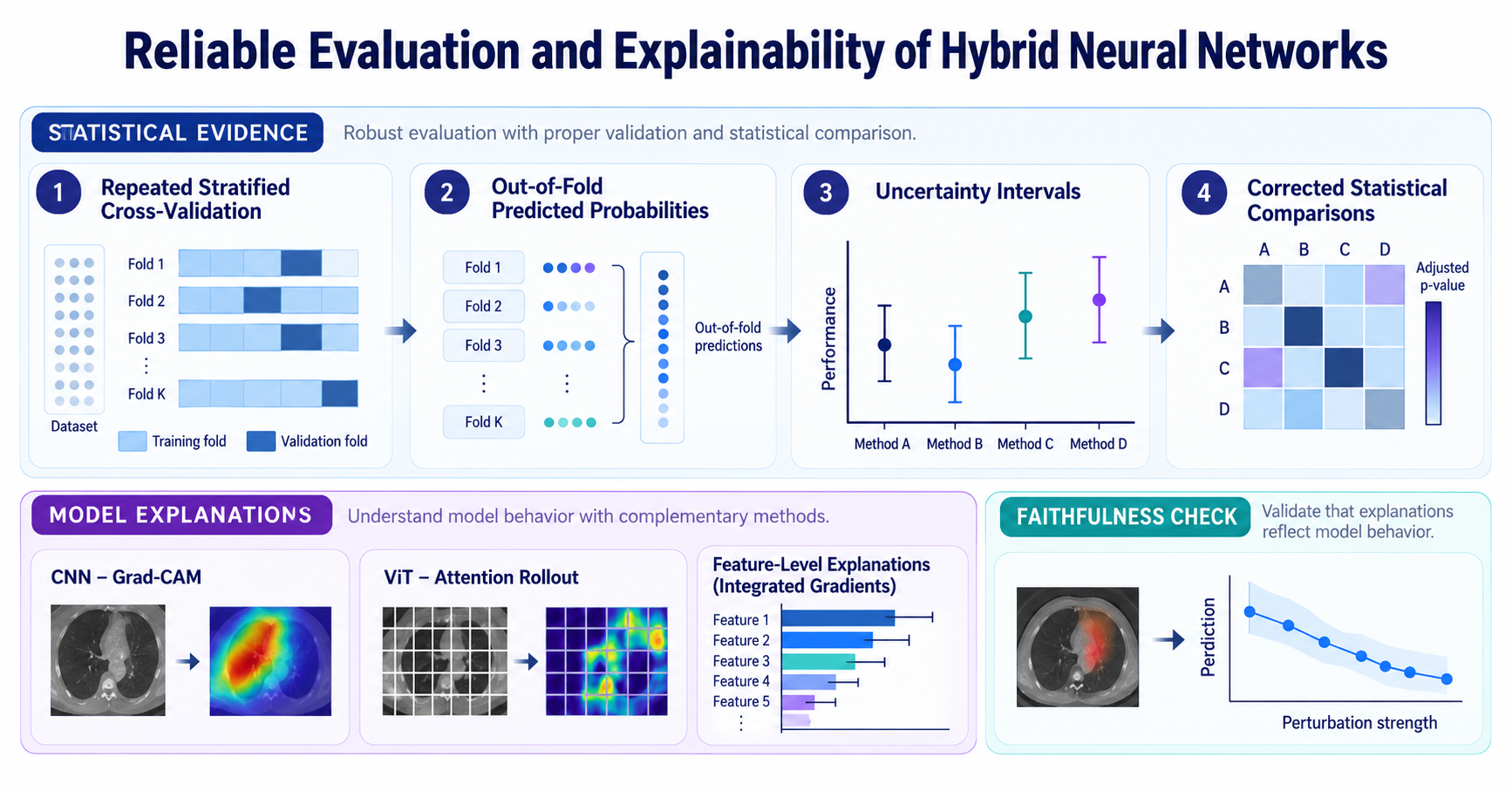
This concluding tutorial follows source notebook sections 10–14. It examines repeated stratified cross-validation, out-of-fold predictions and uncertainty, corrected statistical testing, local and global explainability, and feature-removal experiments.
Reproducibility note. The code fragments in this article continue directly from the definitions in Part I. To run them end-to-end, execute the complete original notebook in section order. The recorded outputs below are preserved as provided, without new experiments.
10. Reliable evaluation
Section 9 answered “does the pipeline work?”. A paper, a thesis or a decision needs a different question answered: “how well will each model perform on new patients, and are the differences between models real?”. This section answers it with the same train/validation/test logic, repeated so that every patient is used for testing and the uncertainty can be quantified.
10.1. Why one split is not enough
A quick experiment makes the problem visible. We take the two tabular baselines, which train in milliseconds, and repeat the 70/15/15 split of Section 3 with 100 different random seeds. The data, the models and the code are identical; only the split changes.
N_LOTTERY = 100
lottery = []
for s in range(N_LOTTERY):
    tr, rest = train_test_split(df, test_size=0.30, stratify=df["target"], random_state=s)
    _, te = train_test_split(rest, test_size=0.50, stratify=rest["target"], random_state=s)
    sc = MinMaxScaler().fit(tr[FEATURES])
    X_tr, X_te = sc.transform(tr[FEATURES]), sc.transform(te[FEATURES])
    for name, clf in [(LOGREG, LogisticRegression(max_iter=5000)), (GBOOST, HistGradientBoostingClassifier(random_state=SEED))]:
        p = clf.fit(X_tr, tr["target"]).predict_proba(X_te)[:, 1]
        lottery.append({"seed": s, "model": name, **metrics(te["target"].to_numpy(), p)})
lottery = pd.DataFrame(lottery)
lr_runs = lottery[lottery["model"] == LOGREG]

fig, axes = plt.subplots(1, 3, figsize=(12, 2.9))
for ax, m in zip(axes, [ACC, AUC, BRIER]):
    ax.hist(lr_runs[m], bins=15, color=TEAL, alpha=0.85)
    ax.axvline(baseline_results[0][m], color=ORANGE, lw=2, label="split of Section 3")
    ax.set_title(f"{LOGREG}: {m}"); ax.set_xlabel(m)
axes[0].set_ylabel("random splits"); axes[0].legend(fontsize=8)
plt.tight_layout()
plt.show()

wide = lottery.pivot(index="seed", columns="model", values=ACC)
print(f"{LOGREG}: test accuracy over {N_LOTTERY} splits: min {lr_runs[ACC].min():.3f}, "
      f"max {lr_runs[ACC].max():.3f}, central 95% [{lr_runs[ACC].quantile(0.025):.3f}, {lr_runs[ACC].quantile(0.975):.3f}]")
print(f"Gradient boosting beats logistic regression in {(wide[GBOOST] > wide[LOGREG]).mean():.0%} of the splits, ties in "
      f"{(wide[GBOOST] == wide[LOGREG]).mean():.0%} and loses in {(wide[GBOOST] < wide[LOGREG]).mean():.0%}.")
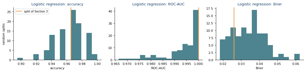
(How changing the train/test split affects estimated accuracy for the same tabular baseline models.)
Notebook output:
Logistic regression: test accuracy over 100 splits: min 0.895, max 1.000, central 95% [0.919, 0.994]
Gradient boosting beats logistic regression in 37% of the splits, ties in 21% and loses in 42%.
Same model, same data, only the split changes: the test accuracy of logistic regression ranges from 0.895 to 1.000 (central 95%: 0.919–0.994), and our split (0.965, orange line) is just one draw. Even the winner changes: gradient boosting beats logistic regression in 37% of the splits, ties in 21% and loses in 42%. No difference between models smaller than this spread can be attributed to the models. With 569 patients a larger test set would starve training, so the standard solution is to use every patient for testing in turn (cross-validation) and quantify the uncertainty explicitly.
10.2. Protocol: repeated stratified cross-validation
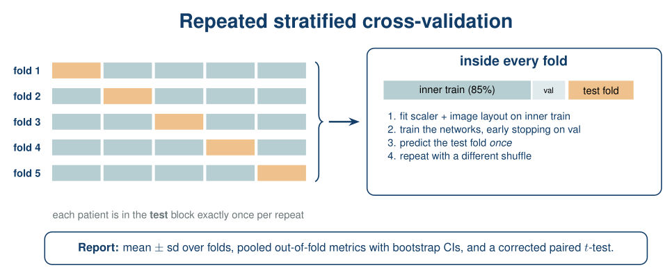
Figure 7. Repeated stratified cross-validation. In every repeat the patients are shuffled and divided into five stratified folds; each fold is the test set once. Inside every fold, an inner validation partition is held out for early stopping, and everything that is learned (scaler, image layout, network weights) uses the inner training partition only.
| Design decision | Choice | Reason |
|---|---|---|
| Outer resampling | RepeatedStratifiedKFold, 5 folds × 2 repeats = 10 train/test partitions | every patient is tested once per repeat; stratification keeps 37% malignant in every fold; repeats average out the luck of one shuffle |
| Inner validation | 15% of each outer training set, stratified | used only for early stopping of the networks |
| What is fitted per fold | scaler, IGTD layout, pixel footprints and the scale check of Section 7.1, network weights | all on the inner training partition: the test fold never influences any learned quantity |
| Baselines | trained on the whole outer training set (inner train + validation) | they need no early stopping; every model sees the same outer training patients |
| Hyperparameters | fixed in advance (Section 9.1) | if you tune them, the search must run inside each outer training set (nested cross-validation), never on the test folds |
| Pairing | same folds and same seed for all models in a fold | differences between models can be analysed fold by fold (paired design) |
| Primary metric | Brier score, declared before running | proper scoring rule, sensitive to calibration, does not saturate like ROC-AUC; balanced accuracy is the secondary metric |
Why the Brier score and not the log-loss?
Both are proper scoring rules, but our networks are trained with label smoothing 0.05, which caps their confidence at about 0.975. That adds a floor of −ln 0.975 ≈ 0.025 to the log-loss of every correctly classified patient, a penalty that the baselines do not pay. The same cap adds only 0.025² ≈ 0.0006 to the Brier score, so the comparison remains fair.
10.3. Running the protocol
The first cell prepares one fold: it splits the outer training set, fits the scaler and a fresh IGTD on the inner training partition, computes the footprints of that fold’s layout and puts every partition on the training scale with restore_scale() (Section 7.1), checking that the restoration is exact.
N_SPLITS, N_REPEATS = 5, 2          # 10 train/test partitions; use more repeats for a final paper
VAL_SIZE = 0.15                     # inner validation, used only for early stopping
MAX_RESTORE_ERROR = 0.01            # tolerance of the scale check of Section 7.1
MODEL_COL = "model"
MODEL_ORDER = [LOGREG, GBOOST, "CNN", "ViT", "HyCNN", "HyViT"]

def make_fold_data(train_idx, test_idx, seed):
    outer = df.iloc[train_idx]
    inner, val = train_test_split(outer, test_size=VAL_SIZE, stratify=outer["target"], random_state=seed)
    splits = {"train": inner.reset_index(drop=True), "val": val.reset_index(drop=True),
              "test": df.iloc[test_idx].reset_index(drop=True)}
    # Everything that is learned is fitted on the inner training partition only
    fold_scaler = MinMaxScaler().fit(splits["train"][FEATURES])
    tab = {s: fold_scaler.transform(d[FEATURES]).astype(np.float32) for s, d in splits.items()}
    method = make_method(seed)
    raw_fold = to_images(method, "cv_fold", splits, verbose=False)
    fold_masks = feature_footprints(method, splits["train"])
    img, worst_error = {}, 0.0
    for s in splits:
        img[s], best, errors = restore_scale(raw_fold[s], tab[s], fold_masks)
        worst_error = max(worst_error, errors[best])
    if worst_error > MAX_RESTORE_ERROR:
        print(f"  WARNING: scale restoration error {worst_error:.3f} > {MAX_RESTORE_ERROR}")
    y_fold = {s: d["target"].to_numpy() for s, d in splits.items()}
    return {"img": img, "tab": tab, "y": y_fold, "restore_error": worst_error, "masks": fold_masks}

def fit_baselines(data, seed):
    # Baselines need no early stopping: they use the whole outer training set (inner train + validation)
    X_fit = np.vstack([data["tab"]["train"], data["tab"]["val"]])
    y_fit = np.concatenate([data["y"]["train"], data["y"]["val"]])
    lr = LogisticRegression(max_iter=5000).fit(X_fit, y_fit)
    gb = HistGradientBoostingClassifier(random_state=seed).fit(X_fit, y_fit)
    return {LOGREG: lr.predict_proba(data["tab"]["test"])[:, 1], GBOOST: gb.predict_proba(data["tab"]["test"])[:, 1]}
The main loop trains the six models in each of the 10 folds and stores two things: the metrics of every fold and the out-of-fold probability of every patient in every repeat. In our CPU run it took 707 s (about 12 minutes); reduce N_REPEATS to 1 for a quick run, or increase it for a final paper (the time grows linearly).
cv = RepeatedStratifiedKFold(n_splits=N_SPLITS, n_repeats=N_REPEATS, random_state=SEED)
oof = {name: np.full((N_REPEATS, len(df)), np.nan) for name in MODEL_ORDER}   # out-of-fold probabilities
fold_rows = []
t_start = time.time()
for f, (train_idx, test_idx) in enumerate(cv.split(df[FEATURES], df["target"])):
    repeat, fold = divmod(f, N_SPLITS)
    seed = SEED + f
    fold_data = make_fold_data(train_idx, test_idx, seed)
    assert fold_data["img"]["train"].shape[-2:] == (H, W), "the image size must be the same in every fold"
    probs = fit_baselines(fold_data, seed)
    for name, build in BUILDERS.items():
        set_seed(seed)                   # paired design: in a fold, every network starts from the same seed
        model, _ = train(build(), fold_data, seed=seed)
        probs[name] = predict_proba(model, fold_data["img"]["test"], fold_data["tab"]["test"])
    for name, p in probs.items():
        oof[name][repeat, test_idx] = p
        fold_rows.append({"repeat": repeat, "fold": fold, MODEL_COL: name, **metrics(fold_data["y"]["test"], p)})
    print(f"repeat {repeat + 1}/{N_REPEATS} · fold {fold + 1}/{N_SPLITS} · {len(test_idx)} test patients · "
          f"Brier: " + ", ".join(f"{name} {brier_score_loss(fold_data['y']['test'], p):.3f}" for name, p in probs.items())
          + f" · {time.time() - t_start:4.0f} s")

cv_results = pd.DataFrame(fold_rows)
assert not any(np.isnan(v).any() for v in oof.values()), "every patient must be tested once per repeat"
10.4. Performance estimates
We look at the results from two complementary angles:
- Fold level (mean ± standard deviation over the 10 folds): how much the result of one train/test partition varies. The standard deviation is not a confidence interval: folds share most of their training data, so they are not independent.
- Pooled out-of-fold: every patient has exactly one test prediction per repeat, so each metric can be computed on all 569 patients at once and averaged over repeats. A bootstrap over patients (1000 resamples) gives a 95% confidence interval that reflects the finite number of test patients; it does not include the variability due to retraining, which is handled by the tests of Section 10.5.
METRIC_COLS = [BRIER, BACC, AUC, F1, ACC]
KIND_COLOUR = {LOGREG: GREY, GBOOST: GREY, "CNN": TEAL, "ViT": TEAL, "HyCNN": ORANGE, "HyViT": ORANGE}

fig, axes = plt.subplots(1, 2, figsize=(12, 3.6))
for ax, m in zip(axes, [BRIER, BACC]):
    values = [cv_results.loc[cv_results[MODEL_COL] == name, m].to_numpy() for name in MODEL_ORDER]
    ax.boxplot(values, vert=False, widths=0.55, showfliers=False, medianprops={"color": NAVY})
    jitter = np.random.default_rng(SEED)
    for i, (name, v) in enumerate(zip(MODEL_ORDER, values), start=1):
        ax.scatter(v, i + jitter.uniform(-0.15, 0.15, len(v)), s=18, color=KIND_COLOUR[name],
                   edgecolor="white", linewidth=0.4, zorder=3)
    ax.set_yticks(range(1, len(MODEL_ORDER) + 1))
    ax.set_yticklabels(MODEL_ORDER)
    ax.invert_yaxis()
    better = "lower is better" if m == BRIER else "higher is better"
    ax.set_title(f"{m} in each of the {len(values[0])} test folds ({better})")
    ax.set_xlabel(m)
fig.legend(handles=[Patch(color=GREY, label="table"), Patch(color=TEAL, label="image"),
                    Patch(color=ORANGE, label="image + table")],
           loc="lower center", ncol=3, frameon=False, bbox_to_anchor=(0.5, -0.06))
plt.tight_layout()
plt.show()

fold_table = pd.DataFrame({m: cv_results.groupby(MODEL_COL)[m].agg(lambda v: f"{v.mean():.3f} ± {v.std(ddof=1):.3f}")
                           for m in METRIC_COLS}).loc[MODEL_ORDER]
fold_table.index.name = MODEL_COL
print("Mean ± standard deviation over folds")
fold_table
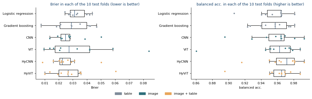
(Fold-to-fold Brier score and balanced accuracy under repeated stratified cross-validation.)
Recorded notebook output (not recomputed for this article):
| model | Brier | balanced acc. | ROC-AUC | F1 (malignant) | accuracy |
|---|---|---|---|---|---|
| Logistic regression | 0.033 ± 0.007 | 0.957 ± 0.022 | 0.994 ± 0.006 | 0.953 ± 0.024 | 0.967 ± 0.016 |
| Gradient boosting | 0.029 ± 0.012 | 0.954 ± 0.020 | 0.991 ± 0.007 | 0.947 ± 0.023 | 0.961 ± 0.016 |
| CNN | 0.027 ± 0.011 | 0.957 ± 0.028 | 0.994 ± 0.006 | 0.952 ± 0.030 | 0.966 ± 0.020 |
| ViT | 0.034 ± 0.023 | 0.955 ± 0.036 | 0.992 ± 0.007 | 0.944 ± 0.042 | 0.960 ± 0.027 |
| HyCNN | 0.025 ± 0.011 | 0.966 ± 0.022 | 0.995 ± 0.006 | 0.958 ± 0.024 | 0.969 ± 0.017 |
| HyViT | 0.028 ± 0.014 | 0.959 ± 0.025 | 0.995 ± 0.005 | 0.951 ± 0.029 | 0.964 ± 0.020 |
N_BOOT = 1000
y_all = df["target"].to_numpy()

# Fast versions of the metrics for the bootstrap (checked against scikit-learn below)
def brier_fast(t, p):
    return np.mean((p - t) ** 2)

def bacc_fast(t, p):
    pred = p >= 0.5
    return 0.5 * (pred[t == 1].mean() + (~pred[t == 0]).mean())

def auc_fast(t, p):
    # Mann-Whitney formulation of ROC-AUC (ties count 1/2)
    r = stats.rankdata(p)
    n1 = t.sum(); n0 = len(t) - n1
    return (r[t == 1].sum() - n1 * (n1 + 1) / 2) / (n1 * n0)

POOLED = {BRIER: (brier_fast, brier_score_loss), BACC: (bacc_fast, balanced_accuracy_score), AUC: (auc_fast, roc_auc_score)}
p_check = oof[LOGREG][0]
for m, (fast, reference) in POOLED.items():
    ref_value = reference(y_all, (p_check >= 0.5).astype(int)) if m == BACC else reference(y_all, p_check)
    assert np.isclose(fast(y_all, p_check), ref_value), m

rng = np.random.default_rng(SEED)
boot_idx = [rng.integers(0, len(y_all), len(y_all)) for _ in range(N_BOOT)]
rows = []
for name in MODEL_ORDER:
    P = oof[name]                                    # (N_REPEATS, patients)
    row = {MODEL_COL: name}
    for m, (fast, _) in POOLED.items():
        point = np.mean([fast(y_all, p) for p in P])
        boot = [np.mean([fast(y_all[i], p[i]) for p in P]) for i in boot_idx]
        lo, hi = np.percentile(boot, [2.5, 97.5])
        row[m] = f"{point:.3f} [{lo:.3f}, {hi:.3f}]"
    rows.append(row)
pooled_table = pd.DataFrame(rows).set_index(MODEL_COL)
print(f"Pooled out-of-fold estimate on {len(y_all)} patients, mean of {N_REPEATS} repeats [95% bootstrap CI]")
pooled_table
Recorded notebook output (not recomputed for this article):
| model | Brier | balanced acc. | ROC-AUC |
|---|---|---|---|
| Logistic regression | 0.033 [0.026, 0.041] | 0.957 [0.937, 0.974] | 0.993 [0.986, 0.998] |
| Gradient boosting | 0.029 [0.019, 0.041] | 0.954 [0.936, 0.971] | 0.990 [0.982, 0.997] |
| CNN | 0.027 [0.019, 0.035] | 0.956 [0.939, 0.973] | 0.993 [0.986, 0.998] |
| ViT | 0.034 [0.023, 0.046] | 0.955 [0.938, 0.970] | 0.987 [0.978, 0.994] |
| HyCNN | 0.025 [0.018, 0.033] | 0.966 [0.951, 0.979] | 0.994 [0.988, 0.998] |
| HyViT | 0.028 [0.018, 0.038] | 0.959 [0.944, 0.974] | 0.991 [0.985, 0.997] |
What the estimates show. All six models are close to the ceiling and their intervals overlap: pooled Brier score from 0.025 (HyCNN) to 0.034 (ViT), balanced accuracy 0.954–0.966 and ROC-AUC 0.987–0.994. The ViT is the least stable model (Brier 0.034 ± 0.023 over folds; in its worst fold, Brier 0.084 and balanced accuracy 0.86), the opposite of what the single split of Section 9 suggested. Descriptively, each hybrid improves on its image-only counterpart (HyCNN 0.025 vs CNN 0.027; HyViT 0.028 vs ViT 0.034); whether these differences are real is tested next.
10.5. Are the differences real? Corrected statistical tests
To compare a model with the reference we use the paired differences of the 10 folds, $d_j = s_j^{\text{model}} - s_j^{\text{ref}}$. A naive paired $t$-test treats the $J$ differences as independent, but the training sets of different folds overlap heavily, so the fold scores are positively correlated and the naive test underestimates the variance and finds too many “significant” differences. The corrected resampled $t$-test (Nadeau & Bengio, 2003), in its repeated cross-validation form (Bouckaert & Frank, 2004), inflates the variance by the ratio of test to training size:
\[t = \frac{\bar d}{\sqrt{\left(\dfrac{1}{J} + \dfrac{n_{\text{test}}}{n_{\text{train}}}\right)\hat\sigma^2_d}}, \qquad \frac{n_{\text{test}}}{n_{\text{train}}} = \frac{1}{k-1}, \qquad \text{df} = J-1,\]with $J = k \cdot r$ folds in total. We fix the reference (logistic regression), the primary metric (Brier) and the significance level (0.05) before looking at the results, and correct for the 5 comparisons per metric with Holm’s method. The table also reports the 95% confidence interval of the mean difference built with the same corrected variance, and the naive $p$-value for comparison.
def corrected_ttest(diff, n_splits=N_SPLITS, level=0.95):
    # Corrected repeated k-fold t-test (Nadeau & Bengio, 2003; Bouckaert & Frank, 2004)
    d = np.asarray(diff, dtype=float)
    J = len(d)
    se = np.sqrt((1 / J + 1 / (n_splits - 1)) * d.var(ddof=1))
    if se == 0:
        return {"mean": d.mean(), "t": np.nan, "p": 1.0 if d.mean() == 0 else np.nan, "lo": d.mean(), "hi": d.mean()}
    t = d.mean() / se
    q = stats.t.ppf(0.5 + level / 2, df=J - 1)
    return {"mean": d.mean(), "t": t, "p": 2 * stats.t.sf(abs(t), df=J - 1),
            "lo": d.mean() - q * se, "hi": d.mean() + q * se}

def holm(pvalues):
    # Holm step-down adjustment for multiple comparisons
    p = np.nan_to_num(np.asarray(pvalues, dtype=float), nan=1.0)
    adjusted, running = np.empty_like(p), 0.0
    for rank, i in enumerate(np.argsort(p)):
        running = max(running, (len(p) - rank) * p[i])
        adjusted[i] = min(1.0, running)
    return adjusted

REFERENCE, ALPHA = LOGREG, 0.05          # fixed before looking at the results
others = [name for name in MODEL_ORDER if name != REFERENCE]
rows = []
for m, lower_is_better in [(BRIER, True), (BACC, False)]:
    per_fold = cv_results.pivot_table(index=["repeat", "fold"], columns=MODEL_COL, values=m)
    tests = [corrected_ttest(per_fold[name] - per_fold[REFERENCE]) for name in others]
    p_holm = holm([t_["p"] for t_ in tests])
    for name, res, p_adj in zip(others, tests, p_holm):
        naive = stats.ttest_rel(per_fold[name], per_fold[REFERENCE]).pvalue
        improves = res["mean"] < 0 if lower_is_better else res["mean"] > 0
        verdict = ("better" if improves else "worse") if p_adj < ALPHA else "no evidence of a difference"
        rows.append({"metric": m, MODEL_COL: name, "mean diff.": res["mean"],
                     "95% CI (corrected)": f"[{res['lo']:+.4f}, {res['hi']:+.4f}]",
                     "p naive": naive, "p corrected": res["p"], "p Holm": p_adj,
                     "verdict": verdict})
tests_table = pd.DataFrame(rows).set_index(["metric", MODEL_COL])
print(f"Differences with respect to {REFERENCE} ({N_SPLITS} folds x {N_REPEATS} repeats)")
tests_table.round(4)
Recorded notebook output (not recomputed for this article):
| metric | model | mean diff. | 95% CI (corrected) | p naive | p corrected | p Holm | verdict |
|---|---|---|---|---|---|---|---|
| Brier | Gradient boosting | -0.0037 | [-0.0148, +0.0074] | 0.1893 | 0.4673 | 1 | no evidence of a difference |
| Brier | CNN | -0.006 | [-0.0136, +0.0016] | 0.0089 | 0.1097 | 0.4387 | no evidence of a difference |
| Brier | ViT | 0.0012 | [-0.0251, +0.0275] | 0.8541 | 0.9217 | 1 | no evidence of a difference |
| Brier | HyCNN | -0.0081 | [-0.0161, -0.0001] | 0.002 | 0.0475 | 0.2376 | no evidence of a difference |
| Brier | HyViT | -0.005 | [-0.0188, +0.0088] | 0.1565 | 0.4299 | 1 | no evidence of a difference |
| balanced acc. | Gradient boosting | -0.0023 | [-0.0187, +0.0140] | 0.561 | 0.7544 | 1 | no evidence of a difference |
| balanced acc. | CNN | -0.0001 | [-0.0181, +0.0179] | 0.9754 | 0.9868 | 1 | no evidence of a difference |
| balanced acc. | ViT | -0.0017 | [-0.0324, +0.0291] | 0.8229 | 0.9047 | 1 | no evidence of a difference |
| balanced acc. | HyCNN | 0.0097 | [-0.0084, +0.0278] | 0.0491 | 0.2552 | 1 | no evidence of a difference |
| balanced acc. | HyViT | 0.0028 | [-0.0189, +0.0245] | 0.6001 | 0.7781 | 1 | no evidence of a difference |
Result. After Holm’s correction, no model differs significantly from logistic regression, in Brier score or in balanced accuracy. The closest case is HyCNN (Brier −0.0081; corrected 95% CI [−0.0161, −0.0001]; corrected p = 0.048, Holm p = 0.24): suggestive, but not evidence once the five comparisons are taken into account.
- The naive test would have misled us: it gives p = 0.002 for HyCNN and p = 0.009 for the CNN. Ignoring the overlap between training sets is one of the most common statistical errors in machine learning papers.
- “No evidence of a difference” is not evidence of equivalence. The ViT interval spans about ±0.027 in Brier score; to claim equivalence, fix in advance the smallest relevant difference (e.g., 0.01) and check that the whole interval lies inside it.
- With 10 folds the tests have limited power; more repeats stabilise the estimates but do not create new patients.
10.6. How to report the results
Reporting checklist. (1) Protocol: repeated stratified cross-validation, inner validation for early stopping, every learned step fitted inside the training folds, hyperparameters fixed in advance, seeds. (2) Estimates with confidence intervals. (3) Primary metric and reference declared in advance; corrected test with multiplicity adjustment. (4) Evidence kept separate from interpretation.
Our results, as they would appear in a paper:
“Under 5×2 repeated stratified cross-validation, the hybrid HyCNN obtained the lowest pooled out-of-fold Brier score (0.025, 95% CI 0.018–0.033) versus 0.033 (0.026–0.041) for logistic regression. After Holm adjustment, the corrected resampled t-test found no evidence of a difference with respect to logistic regression for any model (HyCNN: mean difference −0.008, 95% CI −0.016 to −0.0001; Holm-adjusted p = 0.24).”
Interpretation. On this near-ceiling dataset, image-based and hybrid networks are competitive with, but not demonstrably better than, logistic regression, an honest and legitimate result. The benefits of synthetic images reported in the literature appear mainly with few samples, many features or complex interactions, and must be demonstrated with this same protocol.
11. Explainability for the CNN and the ViT
A model trained on synthetic images is a black box twice over: we must explain the network and translate pixels back into variables. Because we know the footprint of every feature (Section 5), any pixel map can be summed into a per-feature importance (Figure 8). We explain the CNN and the ViT trained on the split of Section 9.
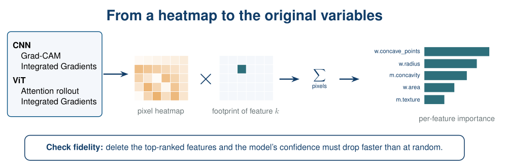
Figure 8. From a heatmap to the original variables. A pixel-level explanation is multiplied by each feature’s footprint and summed, giving one importance value per variable; a deletion test then checks that the ranking is faithful.
11.1. Three explanation tools
| Method | Model | What it shows |
|---|---|---|
| Grad-CAM | CNN | Which regions of the last convolutional maps push the prediction towards the explained class |
| Integrated Gradients (IG) | CNN and ViT | How much each pixel contributes, relative to a reference image (the average training patient) |
| Attention rollout | ViT | Which tokens the [CLS] token draws information from, through all layers |
def per_feature(pixel_map, reduce="sum"):
    # Aggregate a pixel-level map into one value per feature using the footprints
    agg = np.sum if reduce == "sum" else np.mean
    return np.array([agg(pixel_map[m]) if m.any() else 0.0 for m in masks])

def grad_cam(model, img, sign=1.0):
    # Grad-CAM on the output of the CNN's last convolutional stage
    model.eval()
    store = {}
    hook = model.encoder.stage2.register_forward_hook(lambda mod, inp, out: store.update(act=out))
    logit = model(torch.as_tensor(img[None], device=DEVICE))
    hook.remove()
    act = store["act"]
    grad = torch.autograd.grad(sign * logit.sum(), act)[0]
    weights = grad.mean(dim=(2, 3), keepdim=True)            # importance of each channel
    cam = F.relu((weights * act).sum(1, keepdim=True))       # evidence for the explained class
    cam = F.interpolate(cam, size=img.shape[-2:], mode="bilinear", align_corners=False)[0, 0]
    return (cam / (cam.max() + 1e-12)).detach().cpu().numpy()

BASELINE = X_img["train"].mean(0)          # reference input: the average training patient

def integrated_gradients(model, img, steps=64, sign=1.0):
    # IG: average gradient along the straight path from the baseline to the input
    model.eval()
    x = torch.as_tensor(img[None], device=DEVICE)
    b = torch.as_tensor(BASELINE[None], device=DEVICE)
    alphas = (torch.arange(steps, device=DEVICE, dtype=torch.float32) + 0.5) / steps
    path = (b + alphas.view(-1, 1, 1, 1) * (x - b)).requires_grad_(True)
    grads = torch.autograd.grad(sign * model(path).sum(), path)[0]
    return ((x - b) * grads.mean(0, keepdim=True))[0, 0].detach().cpu().numpy()

@torch.no_grad()
def attention_rollout(model, img):
    # Multiply the head-averaged attention matrices of all layers (plus the residual identity)
    model.eval()
    model(torch.as_tensor(img[None], device=DEVICE))
    blocks = model.encoder.blocks
    n = blocks[0].last_attn.shape[-1]
    eye = torch.eye(n, device=DEVICE)
    rollout = eye
    for block in blocks:
        a = block.last_attn[0].mean(0) + eye
        rollout = (a / a.sum(-1, keepdim=True)) @ rollout
    cls_to_tokens = rollout[0, 1:].reshape(model.encoder.grid).cpu().numpy()
    return np.kron(cls_to_tokens, np.ones((PATCH, PATCH)))   # back to pixel resolution
Sanity check: completeness. Integrated Gradients has a useful property: the attributions add up to the change in the model output between the baseline and the input. If the two numbers below are close, the implementation is doing its job.
cnn, vit = models["CNN"], models["ViT"]
x0 = X_img["test"][patient]
for name, model in [("CNN", cnn), ("ViT", vit)]:
    with torch.no_grad():
        f_x = model(torch.as_tensor(x0[None], device=DEVICE)).item()
        f_b = model(torch.as_tensor(BASELINE[None], device=DEVICE)).item()
    ig = integrated_gradients(model, x0)
    print(f"{name}: sum of IG = {ig.sum():+.3f}   |   f(input) - f(baseline) = {f_x - f_b:+.3f}")
Notebook output:
CNN: sum of IG = +8.289   |   f(input) - f(baseline) = +8.271
ViT: sum of IG = +4.184   |   f(input) - f(baseline) = +4.182
Both checks pass: 8.289 vs 8.271 for the CNN and 4.184 vs 4.182 for the ViT (differences below 0.3%, due to the 64-step approximation of the integral).
11.2. Local explanation
We explain the malignant test patient shown in the gallery. Each heatmap is overlaid on the patient’s image, and the bar charts translate the IG maps into the original variables.
maps = {
    "CNN · Grad-CAM": grad_cam(cnn, x0),
    "CNN · Integrated Gradients": integrated_gradients(cnn, x0),
    "ViT · attention rollout": attention_rollout(vit, x0),
    "ViT · Integrated Gradients": integrated_gradients(vit, x0),
}
p_cnn = predict_proba(cnn, x0[None], X_tab["test"][patient:patient + 1])[0]
p_vit = predict_proba(vit, x0[None], X_tab["test"][patient:patient + 1])[0]

fig, axes = plt.subplots(1, 5, figsize=(14, 3.1))
axes[0].imshow(x0[0], cmap="magma", vmin=0, vmax=1, interpolation="nearest")
axes[0].set_title(f"input · P(malignant)\nCNN {p_cnn:.2f} · ViT {p_vit:.2f}")
for ax, (title, m) in zip(axes[1:], maps.items()):
    ax.imshow(x0[0], cmap="gray", vmin=0, vmax=1, interpolation="nearest")
    if "Integrated" in title:
        lim = np.abs(m).max() + 1e-12
        ax.imshow(m, cmap="RdBu_r", vmin=-lim, vmax=lim, alpha=0.8, interpolation="nearest")
    else:
        ax.imshow(m, cmap="inferno", alpha=0.6, interpolation="nearest")
    ax.set_title(title)
for ax in axes:
    ax.set_xticks([]); ax.set_yticks([])
plt.tight_layout()
plt.show()

def short(name):
    return {"mean": "m.", "error": "se.", "worst": "w."}[group_of(name)] + measure_of(name)

fig, axes = plt.subplots(1, 2, figsize=(11, 3.4))
for ax, key in zip(axes, ["CNN · Integrated Gradients", "ViT · Integrated Gradients"]):
    contrib = per_feature(maps[key])
    top = np.argsort(-np.abs(contrib))[:10][::-1]
    ax.barh([short(FEATURES[k]) for k in top], contrib[top],
            color=[ORANGE if contrib[k] > 0 else TEAL for k in top])
    ax.axvline(0, color="grey", lw=0.8)
    ax.set_title(f"{key}: top-10 features\n(orange: towards malignant · teal: towards benign)")
plt.tight_layout()
plt.show()

(Local explanation maps for one held-out test observation: CNN Grad-CAM and Integrated Gradients alongside ViT attention rollout and Integrated Gradients.)
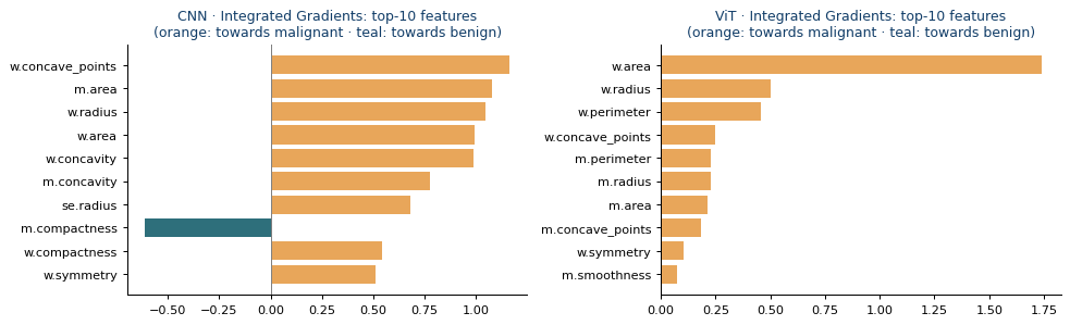
(Feature-level attributions derived from local explanation maps, using the image-to-variable correspondence.)
Both models are confident for this patient (P(malignant) = 1.00 for the CNN and 0.98 for the ViT). The CNN’s evidence comes mainly from size and contour variables (w.concave_points, m.area, w.radius), with m.compactness pushing slightly towards benign; the ViT relies above all on w.area.
- Grad-CAM is coarse: it lives at the resolution of the last convolutional layer (half the input size here) and is then upsampled. It tells you where, not exactly which pixel.
- Integrated Gradients is pixel-exact and signed. With IGTD every 4x4 block is one variable, so the bar chart is a direct reading of the map.
- Attention rollout shows where the ViT routes information. It is not class-specific: attention says what the model looks at, not in which direction it pushes the decision.
11.3. Global explanation
We average the absolute IG contribution of each feature over the whole test set, for both models, and compare the rankings with each other and with the coefficients of the logistic regression baseline.
def global_importance(model):
    return np.mean([np.abs(per_feature(integrated_gradients(model, x, steps=32))) for x in X_img["test"]], axis=0)

imp = {"CNN": global_importance(cnn), "ViT": global_importance(vit)}
coef = np.abs(logreg.coef_[0])

TOP, BOTTOM = 10, 5                       # most and least important variables shown
fig, axes = plt.subplots(1, 2, figsize=(11, 4.8))
for ax, (name, v) in zip(axes, imp.items()):
    order = np.argsort(-v)
    shown = list(order[:TOP]) + list(order[-BOTTOM:])
    ypos = list(range(TOP)) + [TOP + 1 + i for i in range(BOTTOM)]          # a gap separates both groups
    ax.barh(ypos, v[shown], color=[TEAL if name == "CNN" else ORANGE] * TOP + [GREY] * BOTTOM)
    ax.set_yticks(ypos)
    ax.set_yticklabels([short(FEATURES[k]) for k in shown])
    ax.invert_yaxis()
    ax.axhline(TOP, color="grey", lw=0.8, ls=":")
    for yy, k in zip(ypos[TOP:], shown[TOP:]):
        ax.text(v[k], yy, f" {v[k]:.3f}", va="center", fontsize=7.5)
    ax.set_title(f"{name}: mean |IG| per feature (test set)\n{TOP} most and {BOTTOM} least important (grey)")
plt.tight_layout()
plt.show()

print(f"Spearman rank correlation  CNN vs ViT:                       {spearmanr(imp['CNN'], imp['ViT']).correlation:+.2f}")
print(f"Spearman rank correlation  CNN vs |logistic coef.|: {spearmanr(imp['CNN'], coef).correlation:+.2f}")
print(f"Spearman rank correlation  ViT vs |logistic coef.|: {spearmanr(imp['ViT'], coef).correlation:+.2f}")
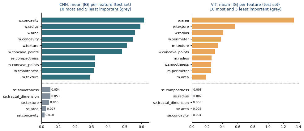
(Global feature-importance profiles across the test set for CNN and ViT, compared with a tabular reference.)
Notebook output:
Spearman rank correlation  CNN vs ViT:                       +0.56
Spearman rank correlation  CNN vs |logistic coef.|: +0.71
Spearman rank correlation  ViT vs |logistic coef.|: +0.75
Reading the global rankings. Both models rely on size and contour variables, and both rankings agree moderately with the logistic regression coefficients (Spearman 0.71 and 0.75) but only partly with each other (0.56): the CNN spreads importance over w.concavity, w.radius, w.area and m.concavity, while the ViT is dominated by w.area.
| The five least important variables are all standard errors (CNN: se.smoothness, se.fractal_dimension, se.texture, se.area, se.concavity; ViT: se.compactness, se.radius, se.fractal_dimension, se.area, se.concavity), with mean | IG | close to zero (≤ 0.054 for the CNN and ≤ 0.008 for the ViT). Some carry almost no class signal, but se.area and se.radius do: they are redundant with the mean and worst values of the same measurement, so the model does not need them. Low importance means “not used by this model”, not “uninformative”. |
Why does w.perimeter appear for the ViT but not for the CNN?
Each chart shows the top 12 of its own model, and for the CNN w.perimeter falls below 12th place. Radius, perimeter and area carry almost the same information (worst radius vs worst perimeter r = 0.993, vs worst area r = 0.985 in the training partition), so a network can use any combination of them, and IG credits the ones that network actually used. Equally good models can therefore split the credit differently. With strongly correlated variables, compare importances by group (e.g., the sum of the IG of radius, perimeter and area), not one by one.
11.4. Are the explanations faithful?
A heatmap is only useful if it reflects what the model really uses. A simple test: remove features one by one, from most to least important, by replacing their pixels with the average training value, and watch how confident the model remains in the true class. If the ranking is faithful, confidence should drop faster than when features are removed in random order. We track confidence rather than ROC-AUC because, on this easy dataset, the AUC stays saturated.
def confidence(model, X):
    # Mean probability the model assigns to the TRUE class of each test patient
    p = predict_proba(model, X, X_tab["test"])
    return np.mean(np.where(y["test"] == 1, p, 1 - p))

def deletion_curve(model, order):
    X = X_img["test"].copy()
    scores = [confidence(model, X)]
    for k in order:
        m = masks[k]
        X[:, :, m] = BASELINE[:, m]          # "delete" feature k: replace it by its average value
        scores.append(confidence(model, X))
    return np.array(scores)

rng = np.random.default_rng(SEED)
fig, axes = plt.subplots(1, 2, figsize=(11, 3.6), sharey=True)
for ax, (name, model) in zip(axes, [("CNN", cnn), ("ViT", vit)]):
    most = deletion_curve(model, np.argsort(-imp[name]))           # most important first
    least = deletion_curve(model, np.argsort(imp[name]))           # least important first
    random_runs = np.array([deletion_curve(model, rng.permutation(len(FEATURES))) for _ in range(5)])
    steps = np.arange(len(most))
    ax.plot(steps, most, color=ORANGE, lw=2, label="most important first (IG)")
    ax.plot(steps, least, color=NAVY, lw=2, ls="--", label="least important first (IG)")
    ax.plot(steps, random_runs.mean(0), color=TEAL, lw=2, label="random order (mean of 5)")
    ax.fill_between(steps, random_runs.min(0), random_runs.max(0), color=TEAL, alpha=0.15)
    ax.set_title(f"{name}: deletion test"); ax.set_xlabel("features removed")
    print(f"{name}: confidence after removing 5 / 10 features -> least important first {least[5]:.3f} / {least[10]:.3f} · "
          f"random {random_runs.mean(0)[5]:.3f} / {random_runs.mean(0)[10]:.3f} · most important first {most[5]:.3f} / {most[10]:.3f} "
          f"(no removal: {most[0]:.3f})")
axes[0].set_ylabel("mean P(true class), test"); axes[0].legend(fontsize=8)
plt.tight_layout()
plt.show()
Notebook output:
CNN: confidence after removing 5 / 10 features -> least important first 0.947 / 0.945 · random 0.937 / 0.897 · most important first 0.881 / 0.733 (no removal: 0.946)
ViT: confidence after removing 5 / 10 features -> least important first 0.965 / 0.965 · random 0.959 / 0.951 · most important first 0.839 / 0.631 (no removal: 0.965)
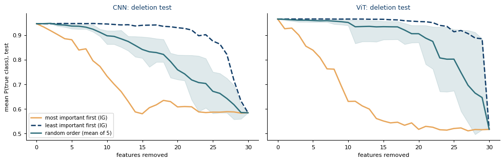
(Faithfulness study based on masking variables according to model attribution, compared with random removal.)
Result. Removing the variables in IG order lowers the confidence in the true class much faster than random removal (after 10 variables: 0.733 vs 0.897 for the CNN and 0.631 vs 0.951 for the ViT), while removing the least important first leaves it practically unchanged (CNN 0.946 → 0.945; ViT 0.965 → 0.965). The two IG curves bracket the random one, which is what faithful rankings should do.
Caveats.
An explanation shows what the model uses, not what causes cancer. IG depends on the baseline (here, the average patient); a black image would tell a different story. These explanations come from one trained model on one split; to check that they are stable, repeat them on the models of several cross-validation folds and compare the rankings. Explanations become harder to trace with blurred or overlapping layouts, which is why methods with a one-to-one pixel-to-feature mapping, such as IGTD or unblurred TINTO, make auditing easier. Always pair heatmaps with a fidelity test such as the deletion curve above.
11.5. Does removing the least important variables help?
The deletion test removes variables from a model that was trained with all of them. A different question is whether a model retrained without the least important variables performs better or worse. Inside each fold of Section 10 we rank the variables with IG on the inner validation partition (never on the test fold, which would be leakage), replace the 5 or 10 least important ones by a constant in every partition, retrain the CNN and the ViT with the same seed and compare them with the full model using the corrected test. Removing the 5 most important variables serves as a contrast. The IGTD layout is kept, so only the information changes, not the image geometry.
# Ablation with retraining: neutralise the k least (or most) important variables, retrain and evaluate.
# The ranking is computed with IG on the inner VALIDATION partition of each fold, never on the test fold:
# choosing variables with test data and then evaluating on the same data would be leakage.
ABL_REPEATS = 1          # 1 -> first 5 folds of Section 10 (about 10 min on CPU); 2 -> all 10 folds (about 20 min)
VARIANTS = {"without 5 least important": ("least", 5),
            "without 10 least important": ("least", 10),
            "without 5 most important": ("most", 5)}           # contrast: removes the strongest evidence
FULL = "all 30 variables"

def ig_importance(model, X, baseline, fold_masks, steps=32):
    # Mean |IG| per variable over the images X, with the fold's own baseline and footprints
    model.eval()
    b = torch.as_tensor(baseline[None], device=DEVICE)
    alphas = (torch.arange(steps, device=DEVICE, dtype=torch.float32) + 0.5) / steps
    total = np.zeros(len(fold_masks))
    for x_np in X:
        x = torch.as_tensor(x_np[None], device=DEVICE)
        path = (b + alphas.view(-1, 1, 1, 1) * (x - b)).requires_grad_(True)
        grads = torch.autograd.grad(model(path).sum(), path)[0]
        attr = ((x - b) * grads.mean(0, keepdim=True))[0, 0].detach().cpu().numpy()
        total += np.abs([attr[m].sum() if m.any() else 0.0 for m in fold_masks])
    return total / len(X)

def neutralise(data, feats, baseline, fold_masks):
    # Replace the selected variables by a constant (training mean) in EVERY partition: they carry no information
    img = {}
    for split, X in data["img"].items():
        X = X.copy()
        for k in feats:
            X[:, :, fold_masks[k]] = baseline[:, fold_masks[k]]
        img[split] = X
    return {**data, "img": img}

def evaluate(model, data):
    p = predict_proba(model, data["img"]["test"], data["tab"]["test"])
    t = data["y"]["test"]
    return {BRIER: brier_score_loss(t, p), BACC: balanced_accuracy_score(t, (p >= 0.5).astype(int))}

abl_rows, least_counts = [], {"CNN": {}, "ViT": {}}
cv = RepeatedStratifiedKFold(n_splits=N_SPLITS, n_repeats=N_REPEATS, random_state=SEED)   # same folds as Section 10
t_start = time.time()
for f, (train_idx, test_idx) in enumerate(cv.split(df[FEATURES], df["target"])):
    repeat, fold = divmod(f, N_SPLITS)
    if repeat >= ABL_REPEATS:
        break
    seed = SEED + f
    fd = make_fold_data(train_idx, test_idx, seed)
    base = fd["img"]["train"].mean(0)
    visible = np.array([k for k, m in enumerate(fd["masks"]) if m.any()])
    for name in ["CNN", "ViT"]:
        set_seed(seed)
        model, _ = train(BUILDERS[name](), fd, seed=seed)
        abl_rows.append({"repeat": repeat, "fold": fold, "model": name, "variant": FULL, **evaluate(model, fd)})
        imp_val = ig_importance(model, fd["img"]["val"], base, fd["masks"])
        order = visible[np.argsort(imp_val[visible])]                   # least important first
        for k in order[:5]:
            least_counts[name][FEATURES[k]] = least_counts[name].get(FEATURES[k], 0) + 1
        for label, (which, n_drop) in VARIANTS.items():
            feats = order[:n_drop] if which == "least" else order[::-1][:n_drop]
            reduced = neutralise(fd, feats, base, fd["masks"])
            set_seed(seed)
            model_r, _ = train(BUILDERS[name](), reduced, seed=seed)
            abl_rows.append({"repeat": repeat, "fold": fold, "model": name, "variant": label, **evaluate(model_r, reduced)})
    print(f"fold {f + 1}/{ABL_REPEATS * N_SPLITS} done · {time.time() - t_start:4.0f} s")

abl = pd.DataFrame(abl_rows)
summary = []
for m in [BRIER, BACC]:
    tests = []
    for name in ["CNN", "ViT"]:
        full = abl[(abl["model"] == name) & (abl["variant"] == FULL)].set_index(["repeat", "fold"])[m]
        for label in VARIANTS:
            red = abl[(abl["model"] == name) & (abl["variant"] == label)].set_index(["repeat", "fold"])[m]
            res = corrected_ttest(red - full)
            tests.append(res)
            summary.append({"metric": m, "model": name, "variant": label, "all 30": full.mean(), "reduced": red.mean(),
                            "mean diff.": res["mean"], "95% CI (corrected)": f"[{res['lo']:+.4f}, {res['hi']:+.4f}]",
                            "p corrected": res["p"]})
    for row, p_adj in zip(summary[-len(tests):], holm([t_["p"] for t_ in tests])):
        row["p Holm"] = p_adj
abl_table = pd.DataFrame(summary).set_index(["metric", "model", "variant"])

for name, counts in least_counts.items():
    ranked = sorted(counts.items(), key=lambda kv: -kv[1])
    print(f"{name}: variables among the 5 least important (folds out of {ABL_REPEATS * N_SPLITS}): "
          + ", ".join(f"{short(v)} ({c})" for v, c in ranked))
print("Brier: lower is better · balanced acc.: higher is better · difference = reduced - all 30")
abl_table.round(4)
Recorded notebook output (not recomputed for this article):
| metric | model | variant | all 30 | reduced | mean diff. | 95% CI (corrected) | p corrected | p Holm |
|---|---|---|---|---|---|---|---|---|
| Brier | CNN | without 5 least important | 0.0292 | 0.0315 | 0.0023 | [-0.0094, +0.0140] | 0.6173 | 1 |
| Brier | CNN | without 10 least important | 0.0292 | 0.0281 | -0.0012 | [-0.0123, +0.0100] | 0.786 | 1 |
| Brier | CNN | without 5 most important | 0.0292 | 0.0285 | -0.0008 | [-0.0168, +0.0153] | 0.9026 | 1 |
| Brier | ViT | without 5 least important | 0.0412 | 0.0331 | -0.0081 | [-0.0271, +0.0109] | 0.3045 | 1 |
| Brier | ViT | without 10 least important | 0.0412 | 0.0374 | -0.0037 | [-0.0172, +0.0098] | 0.487 | 1 |
| Brier | ViT | without 5 most important | 0.0412 | 0.027 | -0.0141 | [-0.0577, +0.0294] | 0.418 | 1 |
| balanced acc. | CNN | without 5 least important | 0.9526 | 0.9476 | -0.0051 | [-0.0539, +0.0438] | 0.7881 | 1 |
| balanced acc. | CNN | without 10 least important | 0.9526 | 0.962 | 0.0094 | [-0.0310, +0.0498] | 0.5541 | 1 |
| balanced acc. | CNN | without 5 most important | 0.9526 | 0.961 | 0.0084 | [-0.0461, +0.0628] | 0.6913 | 1 |
| balanced acc. | ViT | without 5 least important | 0.9458 | 0.9565 | 0.0107 | [-0.0270, +0.0484] | 0.4752 | 1 |
| balanced acc. | ViT | without 10 least important | 0.9458 | 0.9533 | 0.0074 | [-0.0238, +0.0387] | 0.5444 | 1 |
| balanced acc. | ViT | without 5 most important | 0.9458 | 0.9581 | 0.0123 | [-0.0452, +0.0698] | 0.5845 | 1 |
Result. No variant differs significantly from the full model (Holm p = 1.0 in every comparison, 5 folds). Removing the 5 or 10 least important variables changes the Brier score by −0.008 to +0.002, within the fold-to-fold noise: on this near-ceiling dataset, discarding them neither helps nor hurts.
- The contrast is more revealing: removing the 5 most important variables does not hurt either (Brier 0.0285 vs 0.0292 for the CNN). The retrained networks compensate with the remaining, highly correlated variables. IG describes what a trained model uses, not which variables are indispensable for the problem.
- The ViT’s apparent improvements (e.g., 0.0270 vs 0.0412) reflect its instability, with one fold at Brier 0.084 as in Section 10, rather than an effect of the variables; the intervals are wide (up to [−0.058, +0.029]) and 5 folds give little power.
- The least important variables are stable across folds and almost all standard errors: se.smoothness in 5 of 5 folds for the CNN; se.symmetry, se.fractal_dimension, se.compactness and se.concavity in 4 of 5 for the ViT.
- The full models reproduce the Section 10 values for the same folds (CNN 0.029, ViT 0.041), as expected from the fixed seeds.
12. Conclusions
- A synthetic image is a representation choice. TINTOlib offers many, and they expose the same row very differently.
- Fit on training data only, then transform everything else with the frozen method, and check that the same row always gives the same image: a batch-dependent transformation silently shifts validation and test data.
- Hybrid networks keep the exact numbers in an MLP branch while the vision branch exploits the layout; they also recover variables that an image may hide.
- One split is an anecdote, not an estimate. Report repeated cross-validation with every learned step inside the training folds, confidence intervals, and corrected, multiplicity-adjusted tests against strong tabular baselines; declare the primary metric and the reference in advance.
- Explainability must be designed in: use traceable layouts, map pixels back to variables and test the fidelity of the explanations.
- What this notebook found: the best model on the single split (the ViT) is the most variable one under cross-validation, and no network is significantly better than logistic regression on this near-ceiling dataset. The explanations are faithful (deletion test in both directions), but retraining without the least or even the most important variables changes nothing significant: with redundant variables, importance describes the model, not the problem.
13. Exercises
- Another layout. Set
METHOD = "TINTO"in Section 7 and rerun everything, including Section 10. Which features disappear, which hypothesis does Section 7.1 select, and is TINTO better or worse than IGTD according to the corrected test? (Both runs use the same folds and seeds, so the comparison is paired; savecv_resultsbefore rerunning.) - More repeats. Set
N_REPEATS = 5. How do the bootstrap intervals, the corrected confidence intervals and the verdicts change? Why does the width of the bootstrap interval barely change? - Tuning without leakage. Choose the learning rate of the CNN among {1e-3, 5e-4, 2e-4} inside each fold, using only the inner validation partition, and evaluate the selected model on the test fold (nested cross-validation). Compare with the fixed recipe.
- Remove a safeguard. Retrain without label smoothing or without the warm-up. Look at the validation curves of Section 9 and at the Brier score in Section 10: which one tells you more?
- Blurring and Grad-CAM. Train the CNN on
TINTO(..., blur=True)images and compare the Grad-CAM maps with the unblurred version. - Instance-centric images. Feed the CNN with
Clusters(algorithm="kmedoids")images. What does a pixel mean now, and can Section 11 still map it to variables? - Stability of explanations. Keep the CNN of every fold in Section 10 and compute its global IG importance on its own test fold. How stable is the ranking of the top-5 features across folds?
14. References
- TINTOlib. Documentation: https://tintolib.readthedocs.io · Code: https://github.com/oeg-upm/TINTOlib
- TINTOlib crash course (notebooks and videos): https://github.com/oeg-upm/TINTOlib-Crash_Course
- Evaluation and statistics. Nadeau, C. & Bengio, Y. (2003). Inference for the generalization error. Machine Learning, 52(3), 239–281 · Bouckaert, R. R. & Frank, E. (2004). Evaluating the replicability of significance tests for comparing learning algorithms. PAKDD, LNCS 3056, 3–12 · Dietterich, T. G. (1998). Approximate statistical tests for comparing supervised classification learning algorithms. Neural Computation, 10(7), 1895–1923 · Varma, S. & Simon, R. (2006). Bias in error estimation when using cross-validation for model selection. BMC Bioinformatics, 7, 91 · Holm, S. (1979). A simple sequentially rejective multiple test procedure. Scandinavian Journal of Statistics, 6(2), 65–70 · Brier, G. W. (1950). Verification of forecasts expressed in terms of probability. Monthly Weather Review, 78(1), 1–3.
- Explainability. Selvaraju, R. R. et al. (2017). Grad-CAM. ICCV · Sundararajan, M. et al. (2017). Axiomatic attribution for deep networks. ICML · Abnar, S. & Zuidema, W. (2020). Quantifying attention flow in transformers. ACL.
- Blogs & Tutorials: https://www.manuelcastillo.eu/blog/
- Scientific Articles:
- Liu, J., Castillo-Cara, M. y García-Castro, R. (2026). A comprehensive benchmark of spatial encoding methods for tabular data with deep neural networks. Information Fusion, 130, 104088.
- Liu, J., González-Fernández, D., Castillo-Cara, M. y García-Castro, R. (2025). TINTOlib: A Python library for transforming tabular data into synthetic images for deep neural networks. SoftwareX, 32, 102444.
- Castillo-Cara, M. et al. (2025). MIMO-based indoor localisation with hybrid neural networks. IEEE Journal of Selected Topics in Signal Processing, 19(3), 559–571.
- Escalera-González, F., Castillo-Cara, M. et al. (2026). PermGrad: Interpretable hybrid neural networks with synthetic images for tabular data. Knowledge-Based Systems, 350, 116507.
- Mondragon-Ruiz, G., Liu, J., Castillo-Cara, M., & García-Castro, R. (2026). Interpretable CNN–KAN hybrid architectures for tabular data with synthetic image encoding. Information Processing & Management, 63(8), 104954.
- Martínez-Moreno, S., Liu, J., Castillo-Cara, M., Suni-Lopez, F., & García-Castro, R. (2026). CLUSTERS: Instance-Centric Synthetic Images for Tabular Learning and Functional Analysis of Hybrid Fusion.
Where to go next
Return to Part I — From Tabular Data to CNNs, ViTs and Hybrid Models for the image-construction and model-training pipeline.
Continue learning Artificial Intelligence
Explore practical courses on AI, Machine Learning, Deep Learning, Python, R and applied data science.

© Manuel Castillo-Cara, PhD. Content licensed under CC BY-NC 4.0 unless otherwise stated.