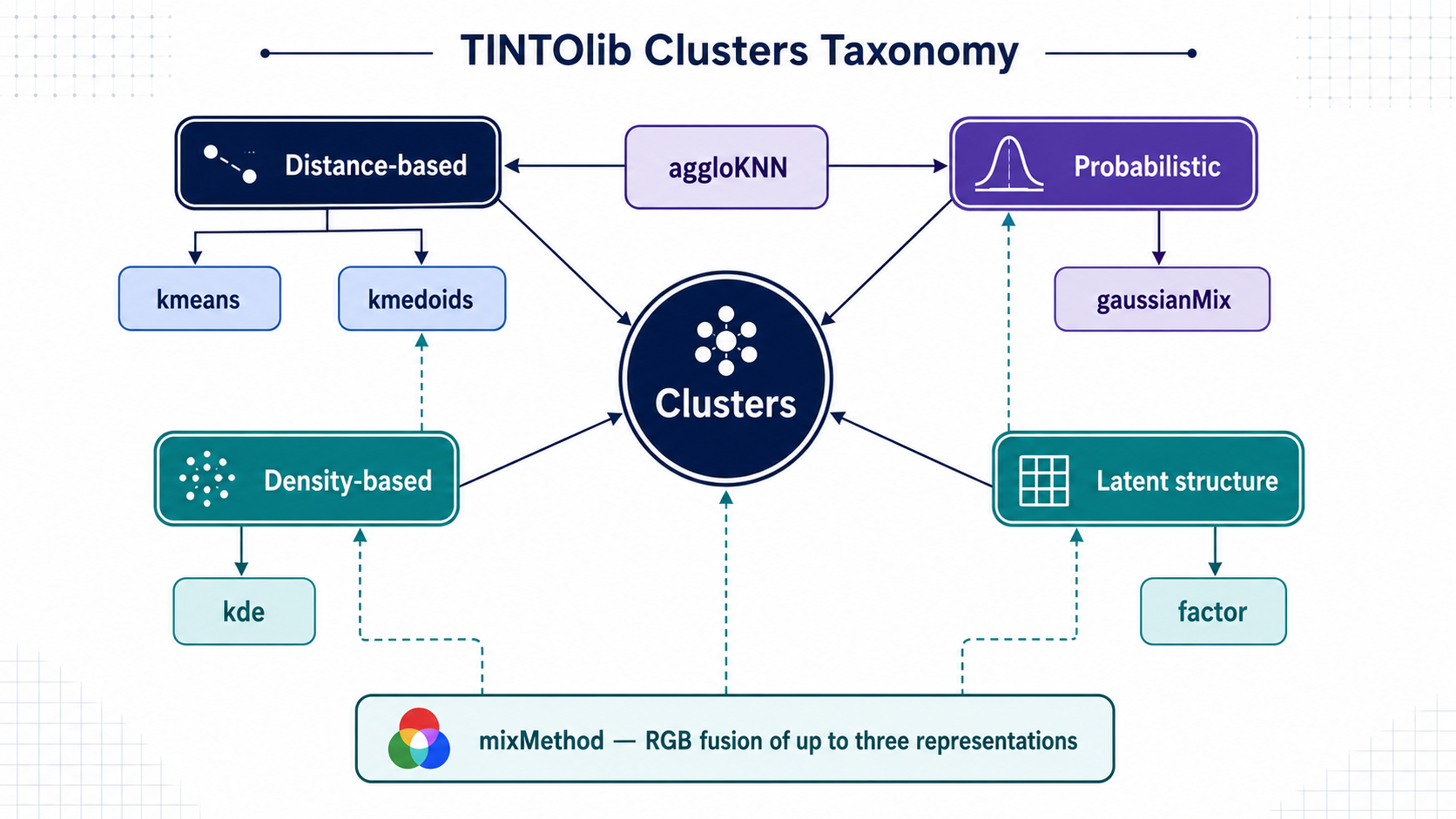
TINTOlib · Clusters · Distance-Based Encodings
k-Means, k-Medoids and aggloKNN
How centroids, representative observations and local connectivity define different intermediate representations before tabular data become synthetic images.
Tutorial metadata
- Author: Manuel Castillo-Cara, PhD
- Affiliation: Dpt. of Artificial Intelligence, Universidad Nacional de Educación a Distancia (UNED), Spain
- Role: Researcher, Professor, and TINTOlib Python Library Developer
- License: CC BY-NC 4.0 unless otherwise stated.
Series note. This is the second article in a four-part series on the unsupervised representations available through the
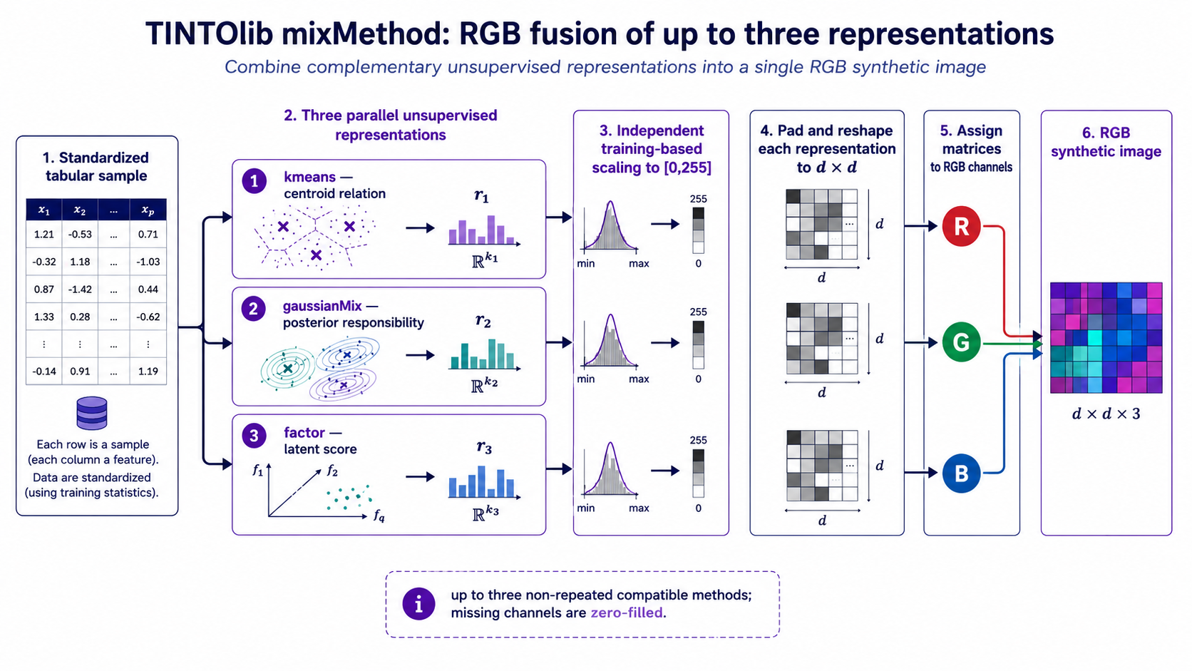
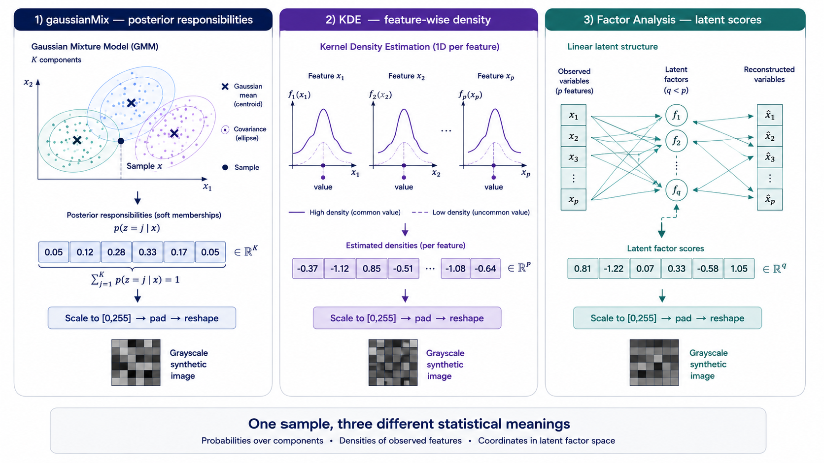
Clustersclass in TINTOlib. Part I introduces the complete family of methods. This post focuses onkmeans,kmedoidsandaggloKNN, while Parts III and IV will examine probabilistic and latent representations, RGB fusion and SSIM-based stability.
Video overview
The following short video summarizes the main concepts introduced in this article.
From cluster assignments to image-ready representations
Clustering algorithms are usually introduced as methods that assign observations to groups. For synthetic image generation, however, a single discrete label contains too little information. If one sample is assigned to cluster 2 and another to cluster 3, the labels alone do not reveal whether the samples are almost identical or located in distant regions of the feature space.
The Clusters class therefore uses richer intermediate representations:
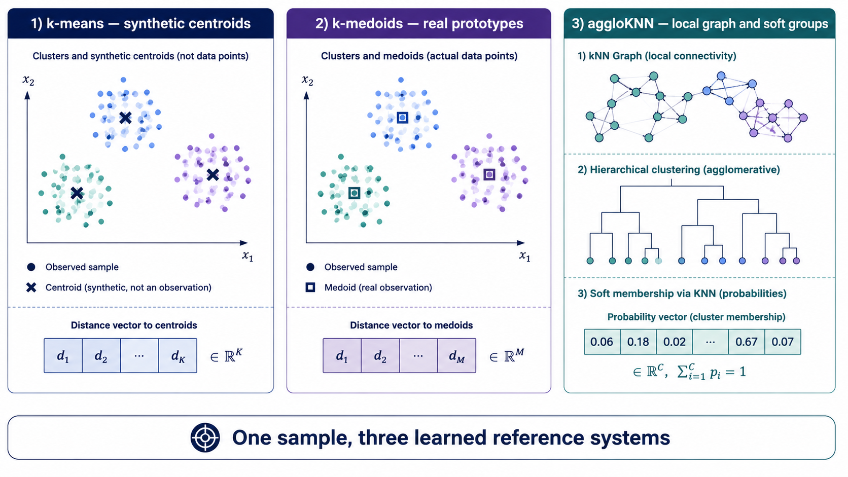
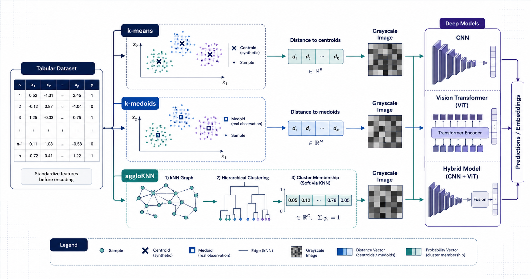
kmeansrepresents each sample through its distances to all learned centroids;kmedoidsuses distances to representative observations selected from the training data;aggloKNNfirst constructs locally constrained hierarchical groups and then converts their pseudo-labels into KNN membership probabilities.
The first two are direct distance encodings. The third is a bridge between distance-based grouping and probabilistic representation: distances define the local graph and the KNN model, while the image pixels contain probabilities rather than raw distances.
This common principle can be expressed as
\[\mathbf{x}_i \in \mathbb{R}^{p} \quad \longrightarrow \quad \mathbf{r}_i \in \mathbb{R}^{k} \quad \longrightarrow \quad \mathbf{I}_i \in \mathbb{R}^{d \times d},\]where $p$ is the number of original variables, $k$ is the number of learned references or groups, and
\[d = \left\lceil \sqrt{k} \right\rceil.\]The vector $\mathbf{r}_i$ is scaled to $[0,255]$, padded when necessary and reshaped into the grayscale image $\mathbf{I}_i$.
 (Figure 1. Three mechanisms for constructing an intermediate representation from tabular samples. k-means uses synthetic centroids, k-medoids selects representative observations from the training data, and aggloKNN combines a local connectivity graph, hierarchical grouping and KNN membership probabilities.)
1. k-Means: distances to synthetic centroids
Let the standardized training set be
\[X = \{\mathbf{x}_1,\ldots,\mathbf{x}_n\} \subset \mathbb{R}^{p}.\]After fitting k-means with $k$ clusters, the method learns centroids
\[\mathbf{c}_1,\ldots,\mathbf{c}_k \in \mathbb{R}^{p}.\]For a cluster $C_j$, its centroid is the arithmetic mean of the samples assigned to that group:
\[\mathbf{c}_j = \frac{1}{|C_j|} \sum_{\mathbf{x}\in C_j}\mathbf{x}.\]TINTOlib does not use only the final cluster label. Instead, every sample is transformed into the complete distance profile
\[\mathbf{r}^{(\mathrm{km})}_i = \left( d(\mathbf{x}_i,\mathbf{c}_1), d(\mathbf{x}_i,\mathbf{c}_2), \ldots, d(\mathbf{x}_i,\mathbf{c}_k) \right).\]This vector describes how the sample relates simultaneously to all regions represented by the centroids. Two samples assigned to different clusters can still have similar distance profiles, while two samples in the same cluster may relate differently to the remaining centroids.
Main parameters
| Parameter | Role |
|---|---|
n_clusters | Number of centroids and therefore initial representation dimensionality |
random_seed | Reproducibility of initialization |
n_init | Number of initial k-means solutions considered |
max_iter | Maximum number of optimization iterations |
algorithmMethod | Scikit-Learn optimization variant: lloyd or elkan |
RBFKmeans | Converts distances into Gaussian similarities before pixel scaling |
In the current implementation, k-means follows its standard Euclidean geometry. Unlike kmedoids and aggloKNN, it does not expose the general metric parameter.
2. k-Medoids: distances to real observations
k-medoids follows the same representational idea but changes the nature of the references. Instead of using arithmetic means, it selects actual observations from the training set:
\[\mathbf{m}_1,\ldots,\mathbf{m}_k \in X.\]Within a cluster $C_j$, the medoid is the observation minimizing the total distance to the other elements in that group:
\[\mathbf{m}_j = \underset{\mathbf{x}\in C_j}{\operatorname{arg\,min}} \sum_{\mathbf{x}'\in C_j} d(\mathbf{x},\mathbf{x}').\]Every sample is then represented by
\[\mathbf{r}^{(\mathrm{kmed})}_i = \left( d(\mathbf{x}_i,\mathbf{m}_1), d(\mathbf{x}_i,\mathbf{m}_2), \ldots, d(\mathbf{x}_i,\mathbf{m}_k) \right).\]Because each medoid is a real training observation, the references can be inspected directly. This can improve the semantic traceability of the representation and may reduce the influence of extreme values compared with mean-based centroids. The trade-off is that the PAM-like iterative search is generally more computationally demanding than k-means.
TINTOlib implements its own PAM-style procedure:
- Select initial medoids from the training observations.
- Assign every sample to the nearest medoid.
- Within each group, identify the observation minimizing the total intra-cluster distance.
- Replace the medoid when a better representative is found.
- Repeat until the medoids remain unchanged or
max_iteris reached.
Supported metrics
The current implementation accepts:
euclidean;manhattan;chebyshev.
The metric affects both cluster construction and the distance profile later converted into the synthetic image.
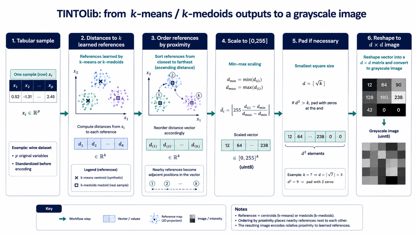 (Figure 2. Distance-vector construction and grayscale image generation for k-means and k-medoids. After learning the references, each sample is represented by its distances to all centroids or medoids. In single-channel mode, TINTOlib reorders these dimensions according to reference proximity before scaling, padding and reshaping the vector into an image.)
Reference ordering and spatial coherence
A list of centroid or medoid distances has no natural two-dimensional order. If its components were reshaped directly, adjacent pixels could correspond to unrelated references.
In grayscale mode, TINTOlib therefore constructs a proximity-based ordering of the learned centroids or medoids before image generation. The procedure starts from a close pair of references and progressively builds a sequence that keeps nearby references close in the one-dimensional vector. The reordered vector is then reshaped into the square image.
This operation does not create a perfect two-dimensional embedding, but it reduces purely arbitrary adjacency and introduces a degree of spatial coherence into the image.
Implementation note. This reference ordering is applied when
kmeansorkmedoidsis used as an individual grayscale method. It is not applied to those methods insidemixMethod, because independently reordering the channels could interfere with their alignment.
RBF smoothing: distances become similarities
Raw distances and local similarities express opposite concepts:
- a small distance indicates proximity;
- a large similarity indicates proximity.
When RBFKmeans=True, TINTOlib transforms the k-means distances using a Gaussian radial basis function:
The implementation estimates $\sigma$ as the global mean of the distance matrix obtained during transformation. Nearby centroids therefore produce values close to one, while distant centroids are progressively attenuated.
The RBF operation changes the representation in three relevant ways:
- Direction of meaning: brighter or larger values can now indicate stronger local affinity rather than greater distance.
- Non-linearity: differences among nearby references are emphasized differently from large-distance differences.
- Visual continuity: the resulting image may show smoother transitions after scaling to pixel intensities.
RBF should not be treated as universally beneficial. It introduces a different inductive assumption and must be assessed as an experimental choice.
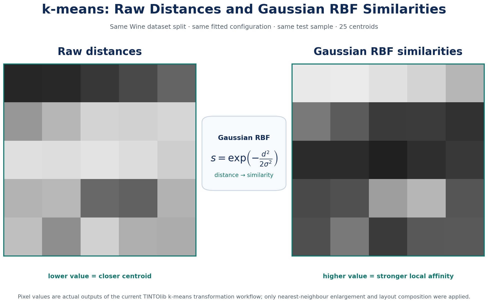 (Figure 3. The same tabular sample represented with k-means before and after Gaussian RBF transformation. The distance image encodes proximity inversely, whereas the RBF image converts distances into bounded similarities that emphasize nearby centroids and attenuate distant references.)
3. aggloKNN: local connectivity followed by soft membership
aggloKNN requires a more precise interpretation. It does not generate pixels directly from the hierarchical-clustering labels. Instead, it combines two stages.
Stage 1: locally constrained agglomerative clustering
The standardized data are first normalized with the L2 norm. A nearest-neighbour connectivity graph is then constructed. In the current implementation, the number of graph neighbours is
\[n_{\mathrm{conn}} = \max\left( 1, \min(10,n-1) \right).\]The graph restricts which observations or groups may be merged during agglomerative clustering. This changes the focus from unrestricted global comparisons to locally admissible connections.
TINTOlib uses complete linkage, where the distance between two groups is determined by the most distant pair of observations across them. The resulting partition provides one pseudo-label for every training sample.
Stage 2: KNN probabilities
The hierarchical model itself does not naturally provide a predict_proba operation for new observations. TINTOlib therefore trains a KNN classifier using the agglomerative labels as pseudo-labels.
The number of neighbours used by this classifier is
\[n_{\mathrm{KNN}} = \max\left( 1, \min(3k,n-1) \right).\]The KNN classifier uses:
- uniform neighbour weights;
- the same selected distance metric;
- brute-force neighbour search.
For each sample, it produces a probability vector
\[\mathbf{r}^{(\mathrm{agg})}_i = \left( P(z=1\mid \mathbf{x}_i), \ldots, P(z=k\mid \mathbf{x}_i) \right).\]Consequently, the final pixels encode soft membership estimates derived from a locally constrained hierarchical partition. This can represent ambiguity near group boundaries more effectively than a single hard cluster label.
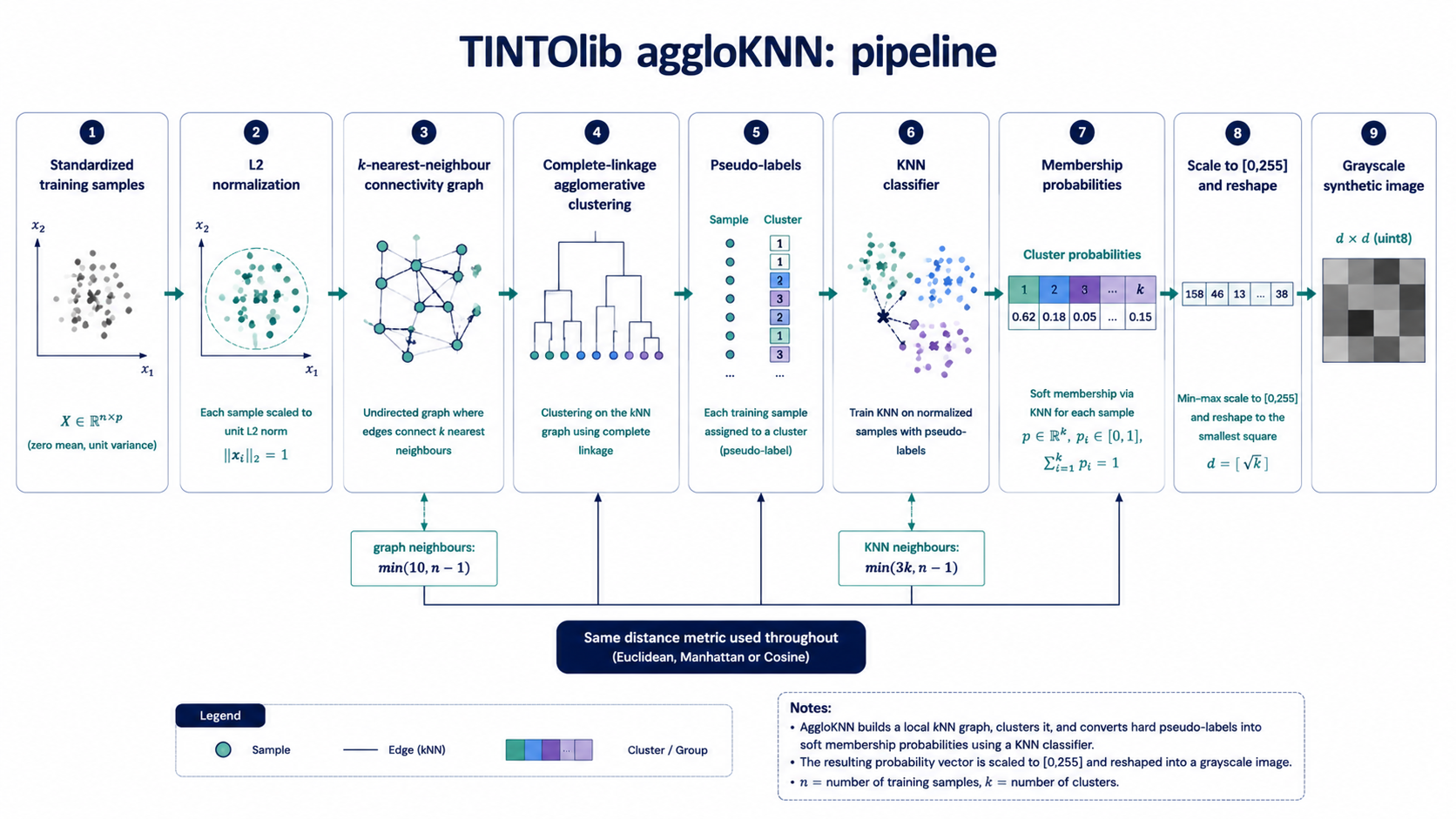 (Figure 4. aggloKNN pipeline. Standardized samples are L2-normalized, connected through a nearest-neighbour graph and grouped with complete-linkage agglomerative clustering. The resulting pseudo-labels train a KNN classifier, whose membership probabilities form the intermediate vector converted into a grayscale synthetic image.)
Supported metrics and current restriction
aggloKNN accepts:
euclidean;manhattan;cosine.
The selected metric is used in the connectivity graph, the agglomerative model and the subsequent KNN classifier.
Unlike kmeans and kmedoids, the current implementation requires an explicit integer for n_clusters. Automatic selection through "auto" or a list of candidates is not currently enabled for aggloKNN.
Comparative view
| Property | kmeans | kmedoids | aggloKNN |
|---|---|---|---|
| Learned references | Synthetic centroids | Real training observations | Locally constrained hierarchical groups |
| Intermediate vector | Distances to centroids | Distances to medoids | KNN membership probabilities |
| Output interpretation | Proximity to mean-based regions | Proximity to representative samples | Soft affinity to pseudo-labelled groups |
| Metric control | Standard k-means geometry | Euclidean, Manhattan or Chebyshev | Euclidean, Manhattan or cosine |
| Optional non-linearity | Gaussian RBF | Not currently available | Not currently available |
| Reference ordering in grayscale | Yes | Yes | No |
Automatic n_clusters selection | Supported | Supported | Not currently supported |
| Main computational concern | Repeated centroid optimization | PAM-style medoid search and pairwise distances | Connectivity graph, hierarchy and KNN probability model |
The table should not be interpreted as a ranking. Each method exposes a different relationship between the original sample and the learned structure of the training set.
Practical implementation with a leakage-free split
The following example generates four representations from the Wine dataset:
- k-means distances;
- k-means RBF similarities;
- k-medoids with Euclidean distance;
- aggloKNN with cosine distance.
The original dataset is split before fitting any transformation.
from pathlib import Path

import pandas as pd
from sklearn.datasets import load_wine
from sklearn.model_selection import train_test_split

from TINTOlib.clusters import Clusters

# ---------------------------------------------------------
# 1. Load a reproducible tabular dataset
# ---------------------------------------------------------
raw_data = load_wine()

df = pd.DataFrame(
    raw_data.data,
    columns=raw_data.feature_names
)

# The target column must be the final column.
df["target"] = raw_data.target

# ---------------------------------------------------------
# 2. Split before fitting the image transformation
# ---------------------------------------------------------
train_df, test_df = train_test_split(
    df,
    test_size=0.20,
    random_state=42,
    stratify=df["target"]
)

# ---------------------------------------------------------
# 3. Define comparable configurations
#    25 references/components -> 5 x 5 images
# ---------------------------------------------------------
models = {
    "kmeans_distances": Clusters(
        problem="classification",
        algorithm="kmeans",
        n_clusters=25,
        random_seed=1,
        n_init="auto",
        max_iter=300,
        algorithmMethod="lloyd",
        RBFKmeans=False
    ),

    "kmeans_rbf": Clusters(
        problem="classification",
        algorithm="kmeans",
        n_clusters=25,
        random_seed=1,
        n_init="auto",
        max_iter=300,
        algorithmMethod="lloyd",
        RBFKmeans=True
    ),

    "kmedoids_euclidean": Clusters(
        problem="classification",
        algorithm="kmedoids",
        n_clusters=25,
        random_seed=1,
        max_iter=300,
        metric="euclidean"
    ),

    "aggloknn_cosine": Clusters(
        problem="classification",
        algorithm="aggloKNN",
        n_clusters=25,
        metric="cosine"
    )
}

# ---------------------------------------------------------
# 4. Fit only on training data and reuse every fitted model
# ---------------------------------------------------------
for name, model in models.items():
    print(f"Generating images with {name}...")

    model.fit(train_df)

    train_folder = Path("synthetic_images") / name / "train"
    test_folder = Path("synthetic_images") / name / "test"

    model.transform(train_df, str(train_folder))
    model.transform(test_df, str(test_folder))

print("Distance-based synthetic images generated successfully.")
With n_clusters=25, each intermediate representation contains 25 values and can therefore be reshaped directly into a $5\times5$ image without zero-padding.
Comparing distance metrics
The metric parameter should be treated as part of the representation design, not merely as an implementation detail.
k-medoids
- Euclidean: emphasizes straight-line geometric distance.
- Manhattan: accumulates absolute coordinate differences and may be appropriate in high-dimensional spaces where axis-wise changes are meaningful.
- Chebyshev: uses the maximum coordinate difference and is therefore controlled by the most discrepant feature.
aggloKNN
- Euclidean: geometric neighbourhoods under L2 distance.
- Manhattan: neighbourhoods based on cumulative absolute differences.
- Cosine: neighbourhoods based primarily on vector orientation after L2 normalization.
Changing the metric may alter:
- the selected medoids;
- the local connectivity graph;
- the agglomerative pseudo-labels;
- the KNN neighbourhoods;
- the final pixel intensities.
A valid metric comparison must therefore refit the transformation independently for every metric while preserving the same train/test partitions.
What should the experiment compare?
The purpose of this post is to explain the representations rather than identify a universally superior method. A rigorous experiment should separate at least four dimensions.
| Evaluation dimension | Questions |
|---|---|
| Representation | How sparse, contrasted or stable are the generated images? How does RBF alter local structure? |
| Prediction | How do the images behave with the same CNN, ViT or hybrid architecture and identical data splits? |
| Robustness | Are conclusions stable across seeds, image resolutions and values of n_clusters? |
| Efficiency | What are the fit time, transform time, memory consumption and generated storage cost? |
The Master’s Thesis used a specific Vision Transformer evaluation architecture. Its results provide evidence for that experimental setting, but they should not be extrapolated directly to CNNs, hybrid tabular–image models or alternative ViT configurations. For that reason, this series does not establish a general ranking among methods.
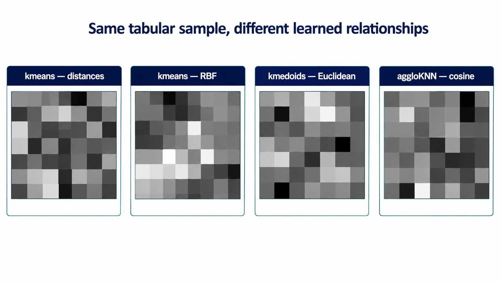 (Figure 5. Synthetic images generated from the same tabular sample using k-means distances, k-means with RBF similarities, k-medoids and aggloKNN. The panels use a common image size, but their pixel semantics differ: centroid distance, centroid similarity, medoid distance and soft membership probability.)
Methodological checklist
Before comparing these transformations, verify that:
- the original split is created before fitting
Clusters; - standardization and all representation models are learned only from training data;
- the same split is reused across methods and metrics;
- image dimensions are controlled through a comparable
n_clustersvalue; - architecture and optimization settings are held constant within each downstream comparison;
- results are repeated across several seeds;
- classical tabular baselines and an MLP remain part of the evaluation;
- conclusions are reported conditionally on the dataset and downstream architecture.
When should each representation be considered?
A reasonable initial interpretation is:
- k-means distances when a computationally efficient reference map based on synthetic centroids is required;
- k-means with RBF when the experiment aims to emphasize local centroid similarity rather than raw distance;
- k-medoids when references tied to real training observations and alternative metrics are relevant;
- aggloKNN when local connectivity, hierarchical grouping and soft membership probabilities are central to the representation.
These are methodological starting points, not performance guarantees.
Conclusion
k-means, k-medoids and aggloKNN begin with a related idea: a tabular sample can be described through its relationship with structures learned from the training set. The nature of that relationship is nevertheless different.
k-means uses distances to synthetic centroids. k-medoids uses distances to representative observations. aggloKNN uses local geometry to construct hierarchical pseudo-labels and then converts those labels into soft KNN probabilities.
These distinctions determine what every pixel means, how the representation responds to distance metrics, whether RBF smoothing is available and how the final image should be interpreted. The correct choice therefore depends on the dataset, the downstream architecture and the experimental objective.
The next post in this series will move from distance-oriented representations to Gaussian Mixtures, Kernel Density Estimation and Factor Analysis, examining probabilities, densities and latent factors as alternative sources of image pixels.
References and resources
Salvador Martínez Moreno. Generación de imágenes sintéticas mediante métodos no supervisados para la librería TINTOlib. Master’s Thesis, Universidad Nacional de Educación a Distancia (UNED), 2026.
TINTOlib documentation. Clusters. Read the current parameter and API documentation.
Research articles
Jiayun Liu, Manuel Castillo-Cara, Raúl García-Castro, Luis Orozco-Barbosa. Interpretable Hybrid Vision Transformer Architectures for MIMO-Based Indoor Localization using Synthetic Spatial Representations. IEEE Internet of Things. DOI: 10.1109/JIOT.2026.3696106
Jiayun Liu, Manuel Castillo-Cara, Raúl García-Castro. A Comprehensive Benchmark of Spatial Encoding Methods for Tabular Data with Deep Neural Networks. Information Fusion. DOI: 10.1016/j.inffus.2025.104088
Giovanny Mondragon-Ruiz, Jiayun Liu, Manuel Castillo-Cara, Raúl García-Castro. Interpretable CNN–KAN hybrid architectures for tabular data with synthetic image encoding. Information Processing and Management. DOI: 10.1016/j.ipm.2026.104954
Felipe Escalera-González, Manuel Castillo-Cara, Mariano Rincón-Zamorano, Luis Orozco-Barbosa. PermGrad: Interpretable Hybrid Neural Networks with synthetic images for tabular data. Knowledge-Based Systems. DOI: 10.1016/j.knosys.2026.116507
Manuel Castillo-Cara, Jesus Martínez-Gómez, Javier Ballesteros-Jerez, Ismael García-Varea, Raúl García-Castro, Luis Orozco-Barbosa. MIMO-Based Indoor Localisation with Hybrid Neural Networks. IEEE Journal of Selected Topics in Signal Processing. DOI: 10.1109/JSTSP.2025.3555067
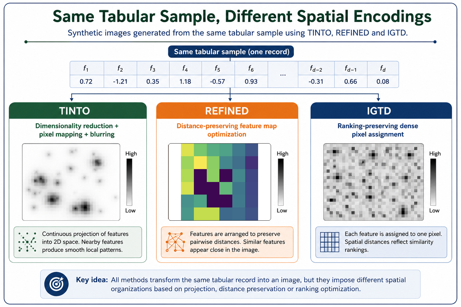
Reewos Talla-Chumpitaz, Manuel Castillo-Cara, Luis Orozco-Barbosa, Raúl García-Castro. Blurring Image Techniques for Bluetooth-based Indoor Localisation. Information Fusion. DOI: 10.1016/j.inffus.2022.10.011
Software articles
Jiayun Liu, David González-Fernández, Manuel Castillo-Cara, Raúl García-Castro. TINTOlib: A Python library for transforming tabular data into synthetic images for deep neural networks. SoftwareX. DOI: 10.1016/j.softx.2025.102444
Manuel Castillo-Cara, Reewos Talla-Chumpitaz, Raúl García-Castro, Luis Orozco-Barbosa. TINTO: Converting Tidy Data into Image for Classification with 2-Dimensional Convolutional Neural Networks. SoftwareX. DOI: 10.1016/j.softx.2023.101391
Continue learning Artificial Intelligence
Explore practical courses on AI, Machine Learning, Deep Learning, Python, R and applied data science.

© Manuel Castillo-Cara, PhD. Content licensed under CC BY-NC 4.0 unless otherwise stated.