TINTOlib · Unsupervised Learning · Synthetic Images
From Clusters to Pixels
How distances, membership probabilities, density estimates and latent factors can be converted into synthetic images for vision-based deep learning.
Tutorial metadata
- Author: Manuel Castillo-Cara, PhD
- Affiliation: Dpt. of Artificial Intelligence, Universidad Nacional de Educación a Distancia (UNED), Spain
- Role: Researcher, Professor, and TINTOlib Python Library Developer
- License: CC BY-NC 4.0 unless otherwise stated.
Series note. This is the first article in a four-part series on the new unsupervised representation methods available through the
Clustersclass in TINTOlib. The series covers distance-based encodings, probabilistic and latent representations, RGB fusion throughmixMethod, and automatic cluster-number selection using SSIM.
Video overview
The following short video summarizes the main concepts introduced in this article.
A new representation family in TINTOlib
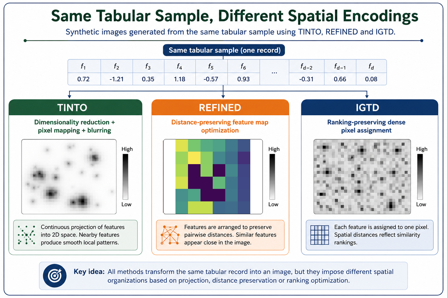
Most tabular-to-image methods begin by asking where the original variables should be placed in a two-dimensional canvas. Methods such as TINTO, REFINED and IGTD construct a spatial organization of features and then project the value of each sample onto that layout.
The new Clusters method introduces a complementary perspective. Instead of directly assigning the original variables to image coordinates, it first learns an intermediate unsupervised representation of every sample. This representation may contain:
- distances to learned centroids;
- distances to representative medoids;
- probabilities of belonging to latent groups;
- estimated probability densities;
- latent factor scores;
- or several of these representations combined across RGB channels.
The resulting numerical vector is subsequently scaled, padded when necessary and reshaped into a square image. Therefore, the image does not directly encode the original columns. It encodes how a sample relates to a set of learned references, distributions or latent structures.
This distinction is important. The method is called Clusters, but not all its internal algorithms are conventional clustering procedures. The class also includes density estimation and latent-factor transformations because all of them can produce structured intermediate representations suitable for image generation.
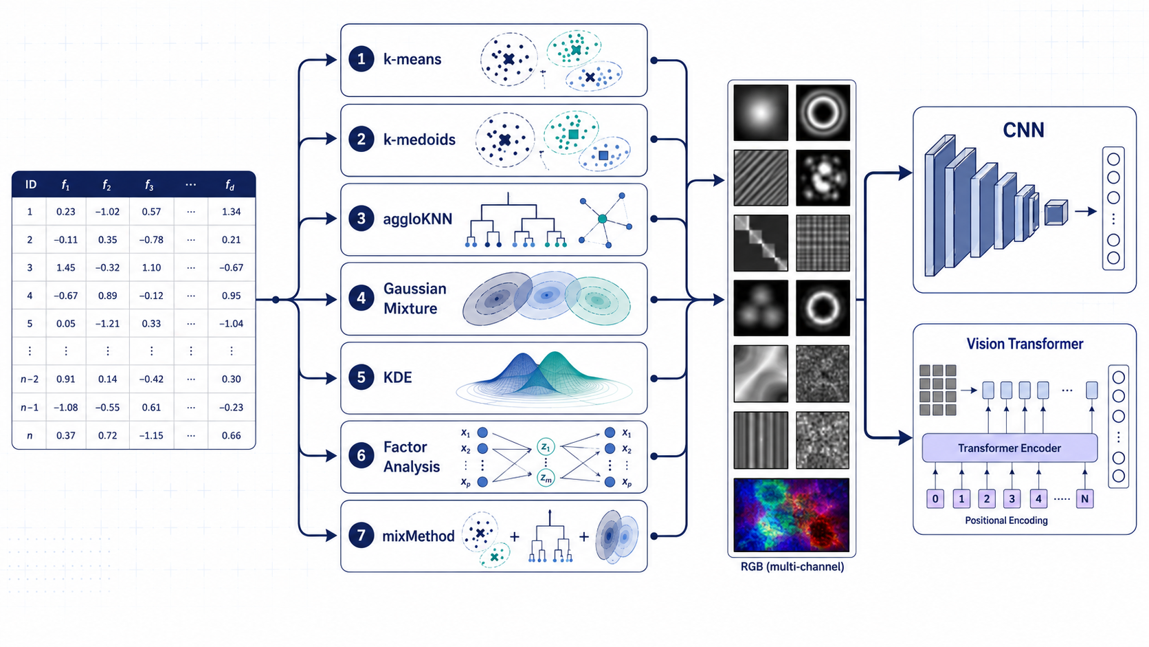 (Figure 1. General workflow of the TINTOlib
 Clusters method. The original tabular data are standardized, transformed into an unsupervised intermediate representation based on distances, probabilities, densities or latent factors, scaled to pixel intensities and reshaped into grayscale or multi-channel synthetic images.)
The central idea: learn a representation before building the image
Let an original tabular sample be represented by
\[\mathbf{x}_i \in \mathbb{R}^{p},\]where $p$ is the number of original variables. The selected unsupervised model learns a transformation
\[\phi: \mathbb{R}^{p} \rightarrow \mathbb{R}^{q},\]and produces an intermediate vector
\[\mathbf{r}_i = \phi(\mathbf{x}_i).\]The meaning of $q$ depends on the selected algorithm. For example, it may be the number of centroids, medoids, Gaussian components or latent factors. In KDE, the dimensionality is tied to the original features because one density estimator is fitted per variable.
The representation $\mathbf{r}_i$ is then transformed into an image through the following operations:
Scale the representation to the range $[0,255]$.
Compute the smallest square side capable of containing all values:
\[d = \left\lceil \sqrt{q} \right\rceil.\]Add zero-padding when $d^2 > q$.
Reshape the vector into a $d \times d$ matrix.
Convert the matrix to an unsigned 8-bit image.
In
mixMethod, repeat the process independently for each selected method and stack the results into the RGB channels.
This design creates a common visual interface for heterogeneous unsupervised models.
Seven algorithms, four representation families
The current implementation supports seven strategies. They can be organized into four conceptual families.
| Family | TINTOlib algorithm | Intermediate representation | Image type | Main parameters |
|---|---|---|---|---|
| Distance-based | kmeans | Distance from each sample to every centroid | Grayscale | n_clusters, n_init, max_iter, algorithmMethod, RBFKmeans |
| Distance-based | kmedoids | Distance from each sample to every medoid | Grayscale | n_clusters, metric, max_iter, random_seed |
| Local probabilistic clustering | aggloKNN | KNN probabilities derived from agglomerative-clustering pseudo-labels | Grayscale | n_clusters, metric |
| Probabilistic mixture | gaussianMix | Posterior probability of every Gaussian component | Grayscale | n_clusters, covariance_type, n_init, max_iter |
| Density-based | kde | Estimated density of every feature value | Grayscale | kernel, bandwidth, metric |
| Latent structure | factor | Factor-analysis scores | Grayscale | n_clusters, random_seed |
| Hybrid multi-view | mixMethod | Up to three representations assigned to R, G and B | RGB | ensamMethod and the parameters required by its component methods |
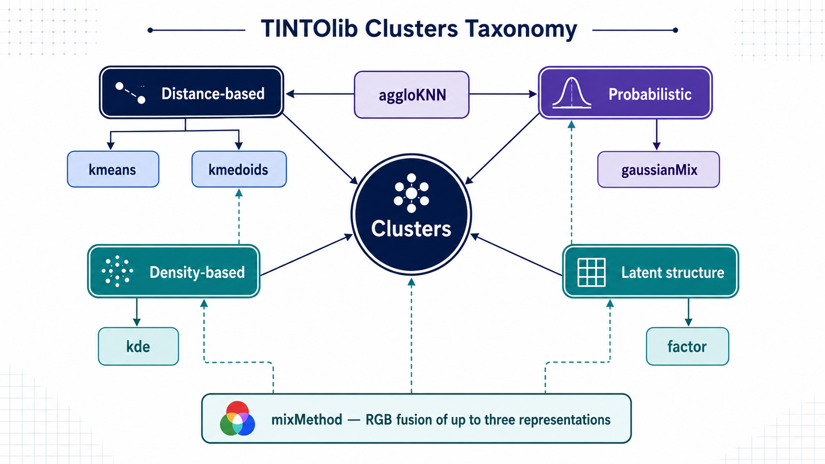
(Figure 2. Conceptual organization of the seven strategies supported by the Clusters class. Distance-based, probabilistic, density-based and latent representations provide different views of the internal structure of tabular data, while mixMethod integrates complementary views into a single RGB image.)
Distance-based representations
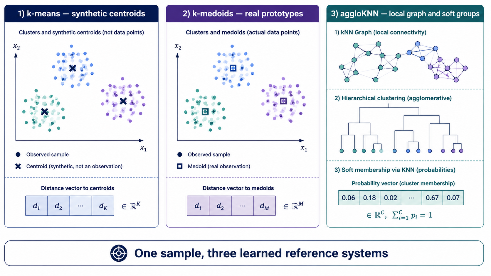
The kmeans and kmedoids variants describe a sample through its distance to a set of learned references. In kmeans, those references are synthetic centroids. In kmedoids, they are real observations selected from the training data.
A distance vector carries more information than a hard cluster label. Two samples assigned to different groups can still have similar distance profiles, and two samples assigned to the same group may relate differently to the remaining clusters.
In grayscale mode, TINTOlib reorders the centroid- or medoid-based dimensions according to reference proximity before reshaping them. The goal is to place related reference regions close to each other in the generated image.
Probabilistic representations
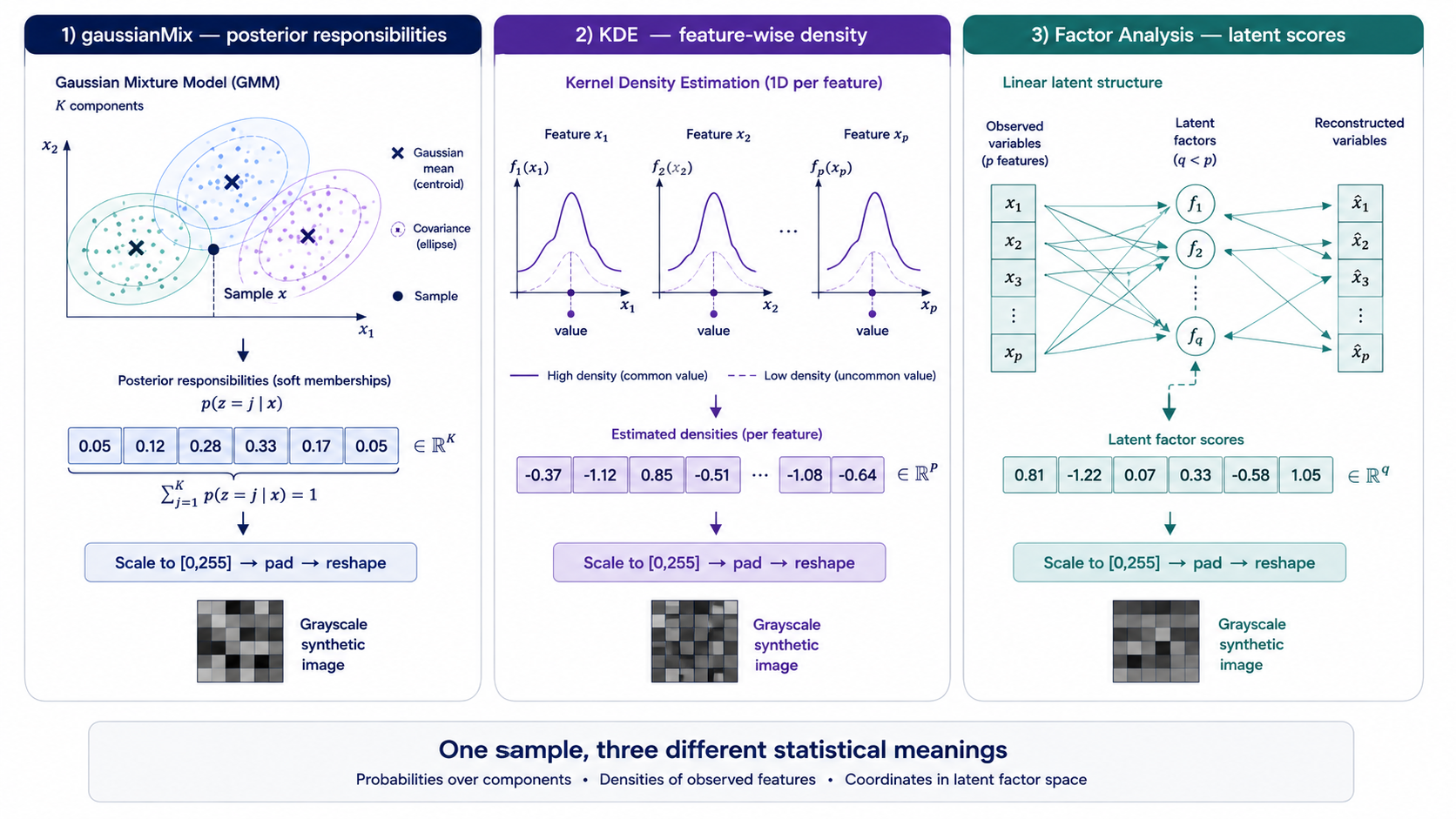
The gaussianMix method replaces distances with posterior membership probabilities. Each pixel indicates the degree to which a sample belongs to one Gaussian component.
The aggloKNN method follows a two-stage procedure. It first applies agglomerative clustering constrained by a nearest-neighbour connectivity graph. The resulting cluster assignments are then treated as pseudo-labels for a KNN classifier, whose probability output becomes the intermediate representation.
Probabilities provide a softer description than hard labels and can capture uncertainty near cluster boundaries.
Density and latent representations
The kde method fits a one-dimensional kernel-density estimator to every feature. Each original value is replaced by its estimated density under the training distribution. The resulting image therefore encodes how common or unusual the values of a sample are, rather than their raw magnitudes.
The factor method projects the original data into a lower-dimensional latent space using Factor Analysis. Its pixels correspond to factor scores that summarize shared variation among the original variables.
Multi-channel representations
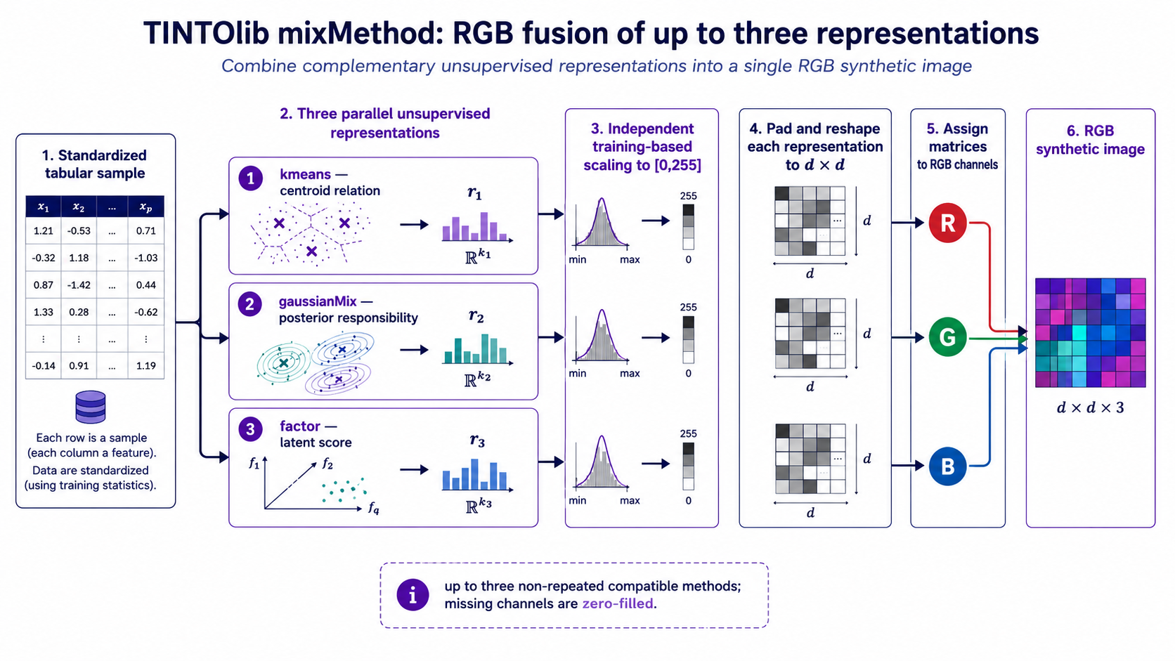
The mixMethod strategy combines between one and three non-repeated methods in an RGB image. Each method fills one colour channel. If fewer than three representations are selected, the remaining channels are filled with zeros.
For example:
- red channel: distances to k-means centroids;
- green channel: Gaussian-mixture membership probabilities;
- blue channel: latent factor scores.
This produces a multi-view image in which colour reflects the interaction among different unsupervised descriptions of the same sample.
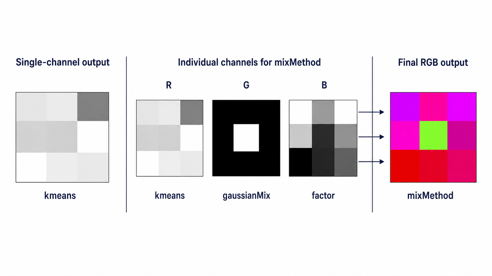 (Figure 3. Comparison between single-channel and multi-channel image generation. Individual methods produce grayscale images, whereas
 mixMethod assigns complementary unsupervised representations to the red, green and blue channels of one synthetic image.)
Why this is different from direct feature-to-pixel mapping
The distinction between spatial feature mapping and cluster-based representation can be summarized as follows.
| Question | Feature-layout methods | Clusters methods |
|---|---|---|
| What is positioned in the image? | Original variables | Learned distances, probabilities, densities or factors |
| What is learned from the training data? | A feature layout or coordinate map | An unsupervised representation model |
| What does a pixel mean? | Value of an original feature at a selected location | Relationship between a sample and a learned reference or latent property |
| Typical image dimensionality | Determined by the number of original features or a chosen canvas | Determined by clusters/components, except KDE |
| Multi-channel option | Method-dependent | Native support through mixMethod |
| Main scientific question | How should related variables be placed? | Which unsupervised description best characterizes each sample? |
Neither paradigm is universally preferable. They encode different inductive assumptions and should be compared under the same leakage-free experimental protocol.
First practical example: k-means with RBF smoothing
The following example uses the Wine dataset from Scikit-Learn. We first divide the data into training and test partitions. The Clusters transformation is then fitted only on the training partition, and the learned model is reused to transform both sets.
from pathlib import Path

import pandas as pd
from sklearn.datasets import load_wine
from sklearn.model_selection import train_test_split

from TINTOlib.clusters import Clusters

# ---------------------------------------------------------
# 1. Load the tabular dataset
# ---------------------------------------------------------
raw_data = load_wine()

df = pd.DataFrame(
    raw_data.data,
    columns=raw_data.feature_names
)

# The target column must be the final column.
df["target"] = raw_data.target

# ---------------------------------------------------------
# 2. Split before fitting the transformation
# ---------------------------------------------------------
train_df, test_df = train_test_split(
    df,
    test_size=0.20,
    random_state=42,
    stratify=df["target"]
)

# ---------------------------------------------------------
# 3. Configure the cluster-based image transformation
# ---------------------------------------------------------
model = Clusters(
    problem="classification",
    algorithm="kmeans",
    n_clusters=25,
    random_seed=1,
    n_init="auto",
    max_iter=300,
    algorithmMethod="lloyd",
    RBFKmeans=True
)

# ---------------------------------------------------------
# 4. Learn the representation from training data only
# ---------------------------------------------------------
model.fit(train_df)

# ---------------------------------------------------------
# 5. Generate training and test images consistently
# ---------------------------------------------------------
train_output = Path("synthetic_images/clusters_kmeans/train")
test_output = Path("synthetic_images/clusters_kmeans/test")

model.transform(train_df, str(train_output))
model.transform(test_df, str(test_output))

print("Cluster-based synthetic images generated successfully.")
With n_clusters=25, every sample is initially represented by 25 distances to the learned centroids. These values fit naturally into a (5 \times 5) image. When RBFKmeans=True, the distance representation is converted into Gaussian radial similarities before pixel scaling, emphasizing nearby centroids and attenuating distant ones.
A useful comparison is to generate the same sample both with and without RBF:
plain_kmeans = Clusters(
    problem="classification",
    algorithm="kmeans",
    n_clusters=25,
    random_seed=1,
    RBFKmeans=False
)

rbf_kmeans = Clusters(
    problem="classification",
    algorithm="kmeans",
    n_clusters=25,
    random_seed=1,
    RBFKmeans=True
)
The first image encodes distances directly; the second emphasizes local similarities.
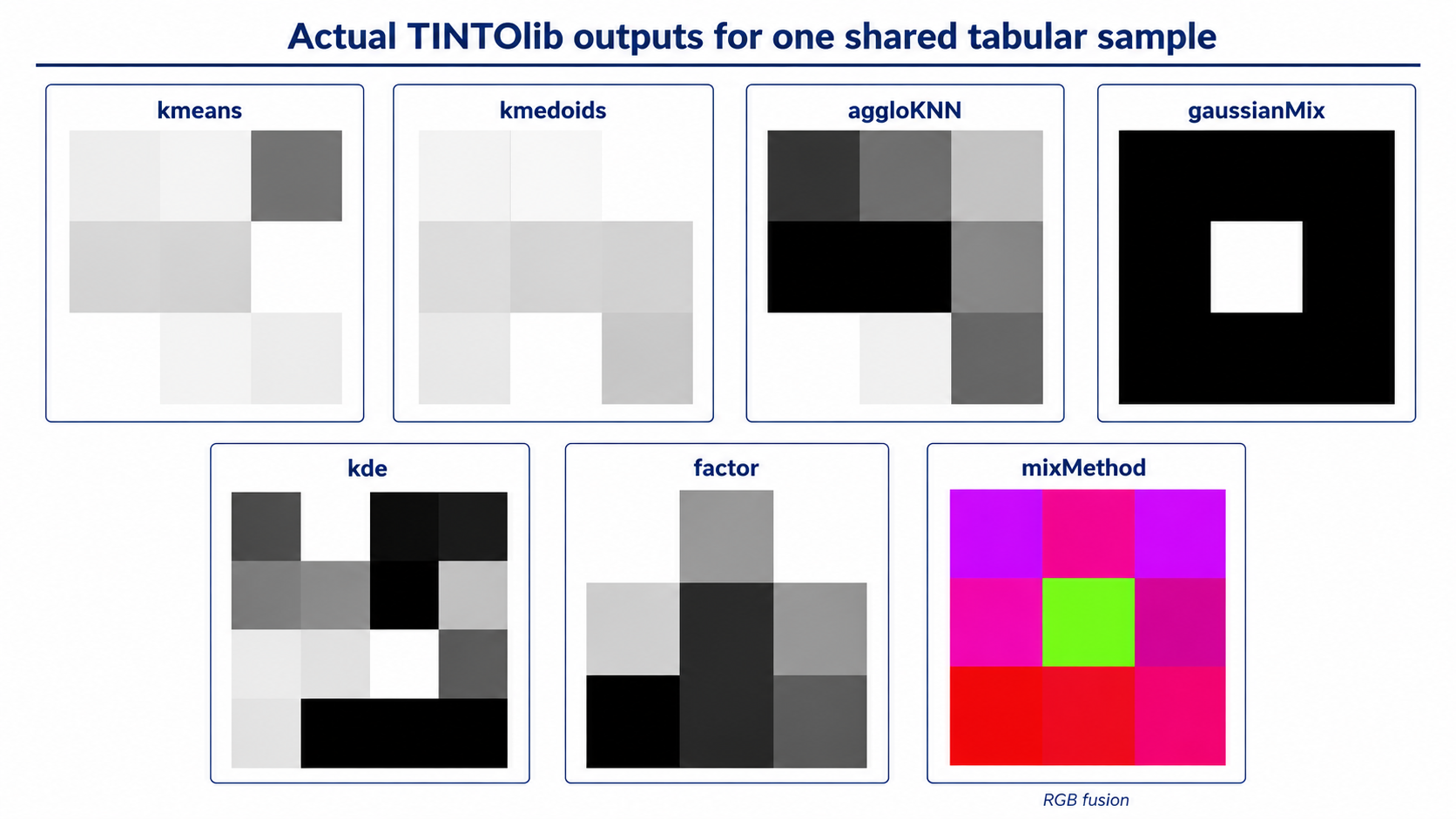 (Figure 4. Representative synthetic images generated from the same tabular sample using
 kmeans, kmedoids, aggloKNN, gaussianMix, kde, factor and mixMethod. The visual differences arise because each algorithm encodes a different intermediate property of the sample: proximity, membership probability, statistical density, latent structure or multi-view fusion.)
Switching between algorithms
TINTOlib uses one class and a common fit/transform workflow. The main change is the algorithm-specific configuration.
models = {
    "kmeans": Clusters(
        problem="classification",
        algorithm="kmeans",
        n_clusters=25,
        RBFKmeans=True
    ),

    "kmedoids": Clusters(
        problem="classification",
        algorithm="kmedoids",
        n_clusters=25,
        metric="euclidean"
    ),

    "gaussianMix": Clusters(
        problem="classification",
        algorithm="gaussianMix",
        n_clusters=25,
        covariance_type="full"
    ),

    "aggloKNN": Clusters(
        problem="classification",
        algorithm="aggloKNN",
        n_clusters=25,
        metric="cosine"
    ),

    "kde": Clusters(
        problem="classification",
        algorithm="kde",
        kernel="gaussian",
        bandwidth=1.0,
        metric="euclidean"
    ),

    "factor": Clusters(
        problem="classification",
        algorithm="factor",
        n_clusters=9,
        random_seed=1
    ),

    "mixMethod": Clusters(
        problem="classification",
        algorithm="mixMethod",
        n_clusters=25,
        ensamMethod=["kmeans", "gaussianMix", "factor"],
        RBFKmeans=True,
        covariance_type="full"
    )
}
Not every parameter applies to every algorithm. The constructor validates incompatible combinations so that configuration errors are detected early.
Parameter compatibility at a glance
| Parameter | kmeans | kmedoids | aggloKNN | gaussianMix | kde | factor | mixMethod |
|---|---|---|---|---|---|---|---|
n_clusters | ✓ | ✓ | ✓ | ✓ | — | ✓ | ✓ |
n_clusters="auto" or list | ✓ | ✓ | — | ✓ | — | ✓ | ✓ |
random_seed | ✓ | ✓ | — | ✓ | — | ✓ | Depends on components |
n_init | ✓ | — | — | ✓ | — | — | Depends on components |
max_iter | ✓ | ✓ | — | ✓ | — | — | Depends on components |
algorithmMethod | ✓ | — | — | — | — | — | When using kmeans |
RBFKmeans | ✓ | — | — | — | — | — | When using kmeans |
covariance_type | — | — | — | ✓ | — | — | When using gaussianMix |
metric | — | ✓ | ✓ | — | ✓ | — | When using applicable components |
kernel / bandwidth | — | — | — | — | ✓ | — | — |
ensamMethod | — | — | — | — | — | — | ✓ |
Current implementation note. Automatic cluster-number selection is not available for
kdeoraggloKNN. KDE does not usen_clusters, andaggloKNNcurrently requires an explicit integer value.
Automatic cluster-number selection with SSIM
For compatible algorithms, n_clusters may be:
- a fixed integer;
- the string
"auto"; - or a list of candidate integers.
When automatic selection is requested, TINTOlib generates representations under several random initializations and evaluates their structural stability using the Structural Similarity Index Measure (SSIM). The selected number of clusters is the one that produces the most stable synthetic images across runs.
For example:
model = Clusters(
    problem="classification",
    algorithm="kmeans",
    n_clusters=[9, 16, 25, 36, 49],
    random_seed=1,
    RBFKmeans=True
)
This is not simply a search for the clustering solution with the lowest internal objective. It evaluates the model from the perspective of the final artifact: the structural consistency of the generated images.
The complete SSIM procedure will be examined in the fourth post of this series.
Methodological note: prevent data leakage
The cluster model, scaling objects, density estimators and latent projections must be learned exclusively from the training partition.
The correct sequence is:
- Split the original tabular data.
- Fit
Clusterson the training set. - Generate training images using the fitted transformation.
- Transform validation and test samples with exactly the same learned objects.
- Train the visual model only on the training images.
- Report performance on untouched validation or test images.
Using fit_transform on the complete dataset before splitting would expose the transformation to the evaluation samples. That can leak information through centroids, medoids, density estimates, Gaussian components, latent factors or scaling ranges.
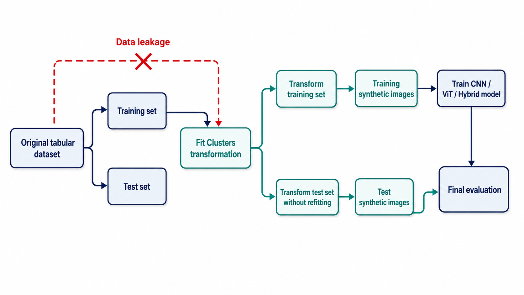 (Figure 5. Leakage-free experimental workflow. The unsupervised representation and its associated scaling operations are fitted only on the training partition and then reused without refitting to generate validation and test images.)
Which representation should I try first?
The following table provides an initial decision guide. It should be treated as a practical starting point, not as a universal ranking.
| Experimental priority | Suggested starting method | Rationale |
|---|---|---|
| Fast and interpretable distance representation | kmeans | Efficient centroid-based encoding with optional RBF smoothing |
| Robust prototypes tied to real observations | kmedoids | Uses actual training samples as cluster representatives |
| Local hierarchical structure and soft assignments | aggloKNN | Combines constrained agglomerative grouping with KNN probabilities |
| Probabilistic cluster membership | gaussianMix | Encodes posterior responsibilities and assignment uncertainty |
| Detect common versus unusual feature values | kde | Converts values into distribution-based density scores |
| Compact latent representation | factor | Encodes shared variability through latent factors |
| Combine complementary descriptions | mixMethod | Places up to three representations in RGB channels |
The transformation should always be assessed together with:
- strong tabular baselines such as XGBoost, LightGBM, CatBoost and Random Forest;
- an MLP trained on the original features;
- several image-based architectures;
- repeated runs and uncertainty estimates;
- computational cost;
- and ablation studies over the main transformation parameters.
How should these methods be evaluated?
The experimental study that motivated these additions evaluated the proposed transformations on regression, binary-classification and multiclass-classification datasets using a specific Vision Transformer architecture. These experiments provide an initial validation of the feasibility of converting unsupervised representations into synthetic images, but they should not be interpreted as a definitive ranking among transformation methods.
A transformation that behaves well with a particular Vision Transformer configuration may exhibit a different behaviour when combined with:
- convolutional neural networks;
- hybrid tabular–image architectures;
- alternative Vision Transformer designs;
- different image resolutions;
- other optimization strategies;
- or datasets with different dimensionality, sample size and feature distributions.
For this reason, the purpose of this series is to present the assumptions, representations, parameters and practical implementation of each method rather than to identify a universally superior alternative.
A rigorous comparison should evaluate every transformation under comparable conditions, include several downstream architectures, report repeated runs and uncertainty estimates, and retain strong classical tabular baselines. The relevant question is therefore not which method is always best, but which representation is most appropriate for a specific dataset, neural architecture and experimental objective.
Roadmap for this four-part series
Part I — From Clusters to Pixels
- Unified conceptual framework.
- Seven supported algorithms.
- Grayscale and RGB image generation.
- First implementation with k-means.
- Leakage-free experimental design.
Part II — Distance-Based Encodings
kmeans,kmedoidsandaggloKNN.- Centroids versus medoids.
- Distance metrics and local connectivity.
- RBF smoothing.
- Side-by-side image and performance comparisons.
Part III — Probabilities, Densities and Latent Factors
gaussianMix,kdeandfactor.- Membership probabilities and covariance structures.
- KDE kernels and bandwidth.
- Factor scores and latent representations.
- When probabilistic encodings become sparse or highly discrete.
Part IV — RGB Fusion and Structural Stability
mixMethodand multi-channel images.- Channel selection and interpretability.
- Automatic
n_clustersselection. - SSIM stability.
- Experimental conclusions, limitations and future directions.
Conclusion
The new Clusters method expands TINTOlib beyond direct feature-layout strategies. Its main contribution is a unified mechanism for turning heterogeneous unsupervised representations into synthetic images.
Distances, membership probabilities, density estimates and latent factors emphasize different aspects of the same tabular sample. Once converted into pixels, these representations can be processed by CNNs, Vision Transformers or hybrid neural networks. However, the transformation itself becomes part of the learning pipeline and must therefore be selected, fitted and evaluated with the same methodological rigor as the downstream predictive model.
The most relevant question is not whether clustering can produce an image. It is whether a particular unsupervised representation preserves information that a visual architecture can exploit more effectively, robustly or interpretably than alternative tabular representations.
References and resources
Salvador Martínez Moreno. Generación de imágenes sintéticas mediante métodos no supervisados para la librería TINTOlib. Master’s Thesis, Universidad Nacional de Educación a Distancia (UNED), 2026.
TINTOlib documentation. Clusters. Read the current parameter and API documentation.
Research articles
Jiayun Liu, Manuel Castillo-Cara, Raúl García-Castro, Luis Orozco-Barbosa. Interpretable Hybrid Vision Transformer Architectures for MIMO-Based Indoor Localization using Synthetic Spatial Representations. IEEE Internet of Things. DOI: 10.1109/JIOT.2026.3696106
Jiayun Liu, Manuel Castillo-Cara, Raúl García-Castro. A Comprehensive Benchmark of Spatial Encoding Methods for Tabular Data with Deep Neural Networks. Information Fusion. DOI: 10.1016/j.inffus.2025.104088
Giovanny Mondragon-Ruiz, Jiayun Liu, Manuel Castillo-Cara, Raúl García-Castro. Interpretable CNN–KAN hybrid architectures for tabular data with synthetic image encoding. Information Processing and Management. DOI: 10.1016/j.ipm.2026.104954
Felipe Escalera-González, Manuel Castillo-Cara, Mariano Rincón-Zamorano, Luis Orozco-Barbosa. PermGrad: Interpretable Hybrid Neural Networks with synthetic images for tabular data. Knowledge-Based Systems. DOI: 10.1016/j.knosys.2026.116507
Manuel Castillo-Cara, Jesus Martínez-Gómez, Javier Ballesteros-Jerez, Ismael García-Varea, Raúl García-Castro, Luis Orozco-Barbosa. MIMO-Based Indoor Localisation with Hybrid Neural Networks. IEEE Journal of Selected Topics in Signal Processing. DOI: 10.1109/JSTSP.2025.3555067
Reewos Talla-Chumpitaz, Manuel Castillo-Cara, Luis Orozco-Barbosa, Raúl García-Castro. Blurring Image Techniques for Bluetooth-based Indoor Localisation. Information Fusion. DOI: 10.1016/j.inffus.2022.10.011
Software articles
Jiayun Liu, David González-Fernández, Manuel Castillo-Cara, Raúl García-Castro. TINTOlib: A Python library for transforming tabular data into synthetic images for deep neural networks. SoftwareX. DOI: 10.1016/j.softx.2025.102444
Manuel Castillo-Cara, Reewos Talla-Chumpitaz, Raúl García-Castro, Luis Orozco-Barbosa. TINTO: Converting Tidy Data into Image for Classification with 2-Dimensional Convolutional Neural Networks. SoftwareX. DOI: 10.1016/j.softx.2023.101391
Continue learning Artificial Intelligence
Explore practical courses on AI, Machine Learning, Deep Learning, Python, R and applied data science.

© Manuel Castillo-Cara, PhD. Content licensed under CC BY-NC 4.0 unless otherwise stated.