TINTOlib · Clusters · Probabilistic and Latent Encodings
Probabilities, Densities and Latent Factors
How Gaussian-mixture responsibilities, per-feature density estimates and latent-factor scores become grayscale synthetic images.
Tutorial metadata
- Author: Manuel Castillo-Cara, PhD
- Affiliation: Dpt. of Artificial Intelligence, Universidad Nacional de Educación a Distancia (UNED), Spain
- Role: Researcher, Professor, and TINTOlib Python Library Developer
- License: CC BY-NC 4.0 unless otherwise stated.
Series note — Part III of IV. This article is the third entry in a four-part technical series on the unsupervised representations available through the TINTOlib
Clustersclass.
- Part I — From Clusters to Pixels: Unsupervised Synthetic Image Generation in TINTOlib
- Part II — Distance-Based Encodings in TINTOlib: k-Means, k-Medoids and aggloKNN
- Part III — Probabilities, Densities and Latent Factors in TINTOlib:
gaussianMix,kdeandfactor— this article.The fourth and final article will examine RGB fusion through
mixMethod, channel interpretation and SSIM-based structural stability.
Video overview
The following short video summarizes the main concepts introduced in this article.
Beyond distances: three alternative views of tabular structure
The distance-oriented methods discussed in Part II describe a sample through its proximity to centroids, medoids or locally constrained groups. The methods examined here answer different questions:
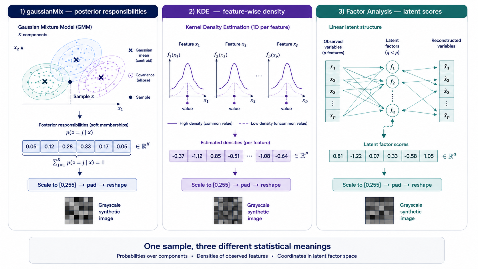
gaussianMix: how strongly does the sample belong to each probabilistic component?kde: how common or unusual is each observed feature value under its training distribution?factor: where is the sample located in a lower-dimensional latent space that explains shared variation among the original variables?
These representations should not be interpreted as interchangeable. Their intermediate vectors have different dimensions, scales and semantics:
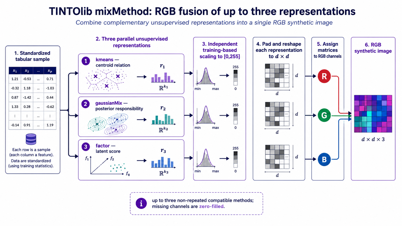
\[\mathbf{x}_i \in \mathbb{R}^{p} \quad \longrightarrow \quad \mathbf{r}_i \quad \longrightarrow \quad \mathbf{I}_i \in \mathbb{R}^{d \times d}.\]For gaussianMix, the representation dimension is the number of Gaussian components, $q=k$. For factor, it is the number of latent factors, $q$. For kde, one estimator is fitted per original feature, so the representation remains $p$-dimensional.
The square side is calculated as
\[d = \left\lceil \sqrt{\dim(\mathbf{r}_i)} \right\rceil,\]and zero-padding is added when the representation does not fill the complete $d \times d$ matrix.
A crucial interpretability distinction must be made. TINTOlib scales the intermediate values to $[0,255]$ using a MinMaxScaler fitted on the training representation. Therefore, the final pixel intensities preserve a relative encoding of the learned representation, but they are not raw calibrated probabilities, densities or signed factor scores.
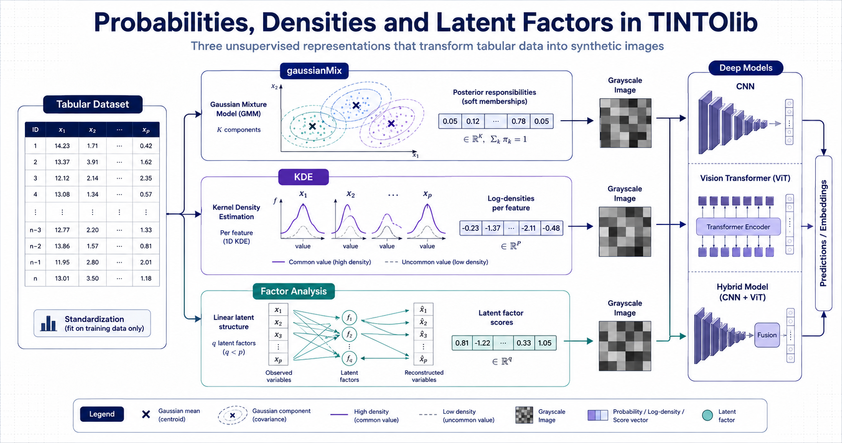 (Figure 1. Three complementary mechanisms for constructing synthetic images from tabular data.
 gaussianMix represents a sample through posterior component responsibilities, kde replaces each feature value with its estimated density under the training distribution, and factor projects the sample onto a lower-dimensional latent space before pixel scaling and reshaping.)
1. gaussianMix: posterior responsibilities as pixels
A Gaussian Mixture Model assumes that the observed data distribution can be approximated by a weighted combination of $k$ multivariate Gaussian components:
\[p(\mathbf{x}) = \sum_{j=1}^{k} \pi_j \mathcal{N} \left( \mathbf{x}\mid\boldsymbol{\mu}_j,\boldsymbol{\Sigma}_j \right),\]where:
- $\pi_j$ is the mixing weight of component $j$;
- $\boldsymbol{\mu}_j$ is its mean vector;
- $\boldsymbol{\Sigma}_j$ is its covariance structure;
- $\sum_{j=1}^{k}\pi_j=1$.
Instead of assigning each sample to only one component, gaussianMix uses the complete posterior responsibility vector:
with
\[\gamma_{ij} = P(z=j\mid\mathbf{x}_i) = \frac{ \pi_j \mathcal{N} \left( \mathbf{x}_i\mid\boldsymbol{\mu}_j,\boldsymbol{\Sigma}_j \right) }{ \sum_{\ell=1}^{k} \pi_\ell \mathcal{N} \left( \mathbf{x}_i\mid\boldsymbol{\mu}_\ell,\boldsymbol{\Sigma}_\ell \right) }.\]Before pixel scaling,
\[\sum_{j=1}^{k}\gamma_{ij}=1.\]The vector therefore describes both component affinity and assignment uncertainty. A sample near the centre of one Gaussian may have one dominant responsibility, whereas a sample near a boundary may distribute its probability mass across several components.
Main parameters
| Parameter | Role |
|---|---|
n_clusters | Number of Gaussian components and intermediate-vector dimensions |
random_seed | Reproducibility of the fitted mixture |
n_init | Number of EM initializations |
max_iter | Maximum EM iterations for each initialization |
covariance_type | Structure imposed on the component covariance matrices |
Implementation note. In the current implementation,
n_init="auto"is converted internally to one Gaussian-mixture initialization. Use an explicit integer such asn_init=5when several EM restarts are required.
Covariance structures
| Value | Covariance assumption | Representational implication |
|---|---|---|
full | Every component has its own complete covariance matrix | Can model component-specific correlations and orientations |
tied | All components share one complete covariance matrix | Different means, but a common covariance geometry |
diag | Every component has its own diagonal covariance | Feature covariances are excluded within each component |
spherical | Every component has one scalar variance | Most constrained and isotropic geometry |
The selected structure changes the learned component geometry and therefore the responsibility vector assigned to each sample.
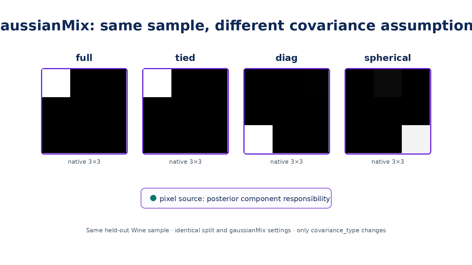 (Figure 2. Synthetic images generated from the same tabular sample using
 gaussianMix with full, tied, diag and spherical covariance structures. Every panel encodes posterior component responsibilities under a different geometric assumption; no configuration should be interpreted as universally preferable.)
Why can Gaussian-mixture images look highly discrete?
It is common for a fitted mixture to assign almost all posterior mass to one component:
\[\mathbf{r}^{(\mathrm{gmm})}_i \approx (0,\ldots,0,1,0,\ldots,0).\]After training-based MinMax scaling, this may produce images dominated by very dark pixels and one or a few bright regions. This is not necessarily an implementation error. It may indicate:
- well-separated Gaussian components;
- a sample located far from component boundaries;
- a covariance constraint that creates confident assignments;
- or an excessive number of components relative to the available data.
Conversely, a more graded image can indicate overlapping components or greater assignment ambiguity. Neither visual pattern guarantees better downstream prediction. The representation must be evaluated together with the dataset and neural architecture.
Another methodological issue is component ordering. Gaussian component indices have no intrinsic semantic order and may be permuted across independently fitted models. Train, validation and test images remain consistent when they are transformed with the same fitted model, but comparisons across independent runs require care.
2. kde: one density estimator per feature
Kernel Density Estimation provides a non-parametric alternative. In the current TINTOlib implementation, a separate one-dimensional KDE model is fitted for every standardized input feature.
For feature $j$, containing training observations
\[x_{1j},x_{2j},\ldots,x_{nj},\]the estimated density can be written as
\[\widehat{f}_j(x) = \frac{1}{nh} \sum_{m=1}^{n} K\left( \frac{x-x_{mj}}{h} \right),\]where:
- $K$ is the selected kernel;
- $h>0$ is the bandwidth;
- $n$ is the number of training samples.
For sample $\mathbf{x}_i$, the intermediate representation is
\[\mathbf{r}^{(\mathrm{kde})}_i = \left( \widehat{f}_1(x_{i1}), \widehat{f}_2(x_{i2}), \ldots, \widehat{f}_p(x_{ip}) \right).\]Each component answers a feature-specific question: how dense is the training distribution around this observed value?
This is not a joint multivariate probability for the complete sample. It is a collection of independent univariate density evaluations.
Main parameters
| Parameter | Role |
|---|---|
kernel | Shape of the local contribution centred on every training observation |
bandwidth | Degree of smoothing applied to the estimated density |
metric | Distance metric used by the KDE estimator |
Supported kernels are:
gaussian;tophat;epanechnikov;exponential;linear;cosine.
Supported metrics are:
euclidean;manhattan;chebyshev.
The implementation obtains log-density scores through score_samples, applies the exponential function and fits a MinMaxScaler on the resulting training densities.
Bandwidth controls the representation scale
The bandwidth is usually the most influential KDE parameter.
- Small bandwidth: narrow local peaks, greater sensitivity to individual observations and potentially fragmented representations.
- Large bandwidth: smoother densities, less local detail and more similar values across broad regions.
A very small bandwidth may classify many test values as lying in low-density regions. A very large bandwidth may suppress potentially meaningful local structure.
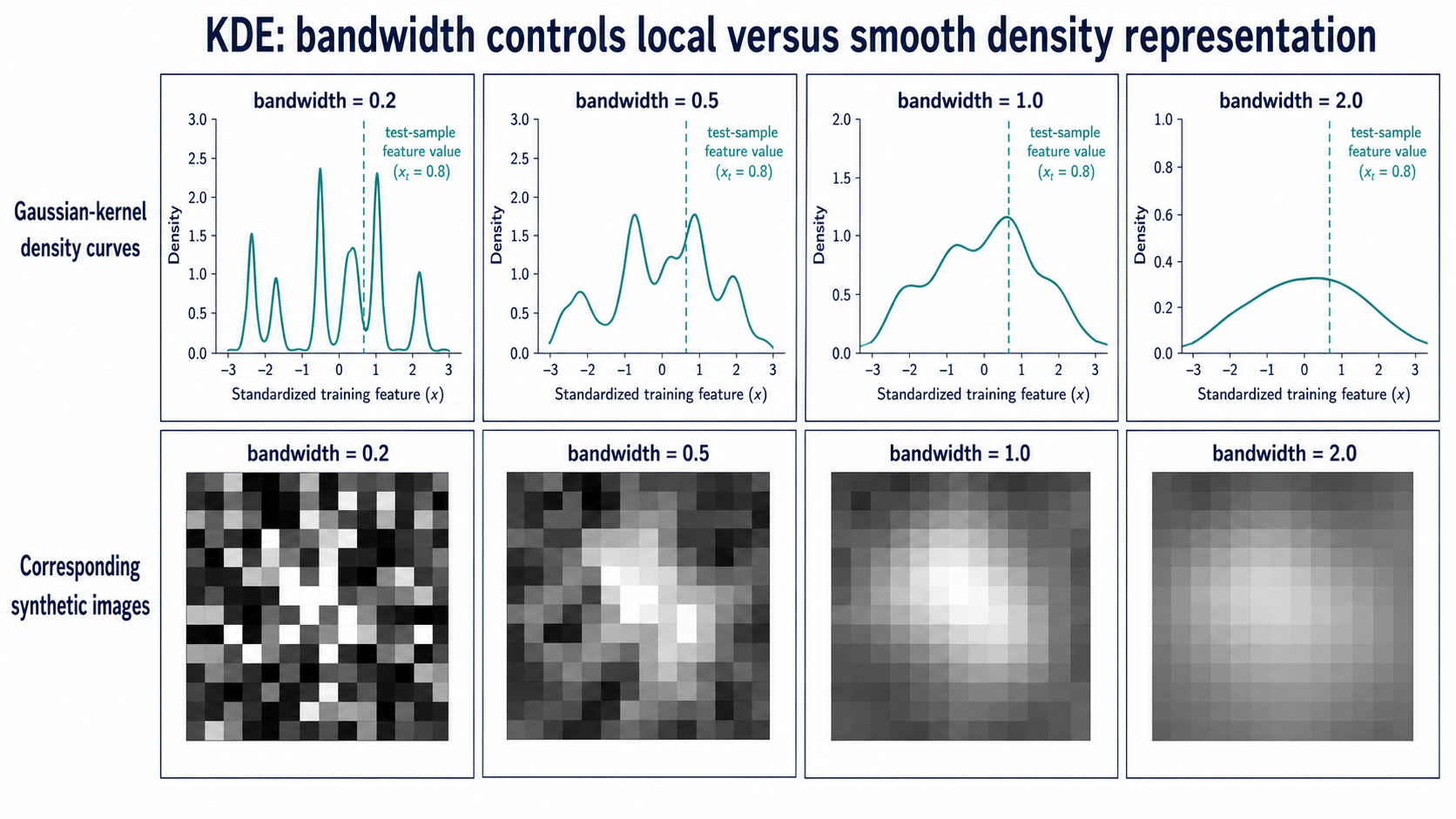 (Figure 3. Effect of kernel shape and bandwidth on the density representation used by
 kde. The curves must be estimated from the same standardized training feature. The associated synthetic-image panels show how local versus smooth density estimates alter the pixel intensities assigned to the same tabular sample.)
Why KDE has a different image size
Unlike the component-based methods, kde does not use n_clusters. Its intermediate vector contains one density value per original feature:
For the Wine dataset, which contains 13 input features,
\[d=\left\lceil\sqrt{13}\right\rceil=4,\]so the resulting image has size $4\times4$, with three padded positions.
This property also explains why kde is not currently available as a channel inside mixMethod: its output dimensionality is determined by the dataset rather than by a shared number of components.
Interpreting KDE pixels
Before scaling:
- a high density indicates that the feature value lies in a common region of its training distribution;
- a low density indicates a locally uncommon or potentially atypical value.
After MinMax scaling, brightness expresses relative density according to the training-derived scaling range. It should not be interpreted as a probability that the complete sample is normal or anomalous.
3. factor: latent scores as a compact image representation
Factor Analysis does not create groups or estimate feature-wise densities. It models the covariance structure of the observed variables through a smaller set of latent factors.
A standard formulation is
\[\mathbf{x}_i = \boldsymbol{\mu} + \mathbf{\Lambda}\mathbf{z}_i + \boldsymbol{\varepsilon}_i,\]where:
- $\mathbf{x}_i\in\mathbb{R}^{p}$ is the observed sample;
- $\boldsymbol{\mu}$ is the feature mean vector;
- $\mathbf{z}_i\in\mathbb{R}^{q}$ is the latent-factor score vector;
- $\mathbf{\Lambda}\in\mathbb{R}^{p\times q}$ is the loading matrix;
- $\boldsymbol{\varepsilon}_i$ represents feature-specific variation not explained by the common factors.
TINTOlib uses the transformed factor scores as the intermediate representation:
\[\mathbf{r}^{(\mathrm{factor})}_i = \mathbf{z}_i = \left( z_{i1}, z_{i2}, \ldots, z_{iq} \right).\]The API retains the parameter name n_clusters, but for factor it means the number of latent factors, not the number of clusters.
Main parameters
| Parameter | Role |
|---|---|
n_clusters | Number of latent factors and output dimensions |
random_seed | Reproducibility of the Factor Analysis fit |
The current implementation requires
\[q \leq p-1.\]For example, a dataset with 13 original features can use at most 12 factors in the current Clusters implementation.
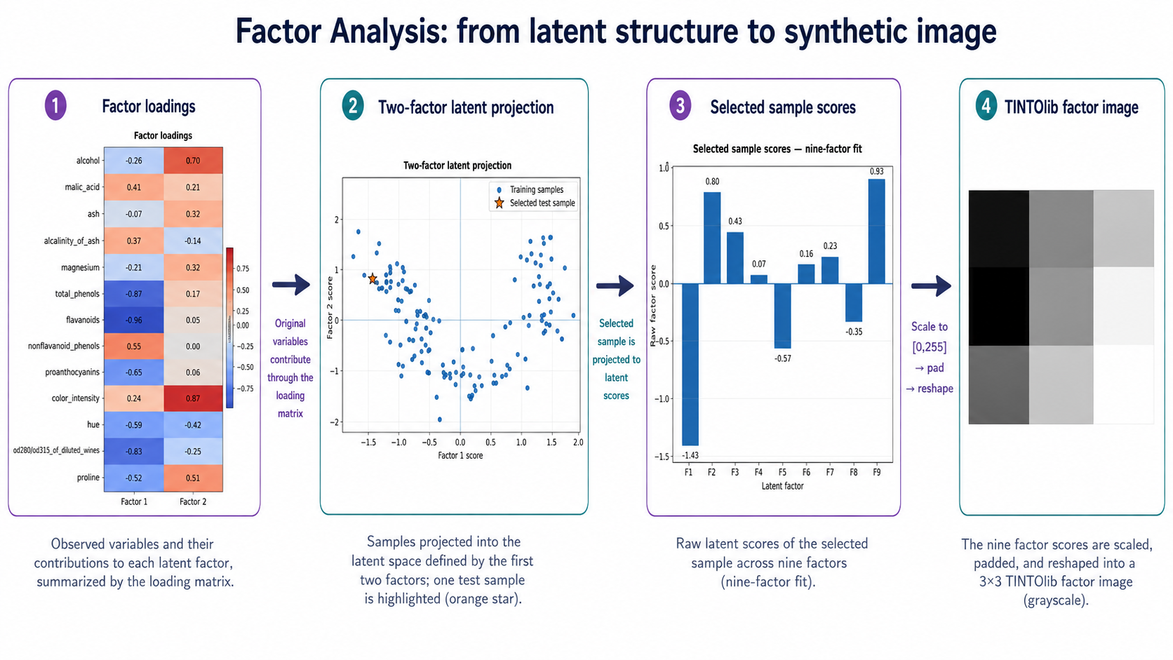 (Figure 4. Factor Analysis representation used by TINTOlib. The fitted loading matrix relates original variables to latent factors, every sample is projected into the factor-score space, and the resulting score vector is scaled and reshaped into a grayscale synthetic image.)
Scores, loadings and pixel meaning
Two quantities must be distinguished:
- factor loadings: describe how the original variables contribute to the latent factors;
- factor scores: describe where each sample lies in the learned latent space.
The image is generated from the factor scores, not directly from the loading matrix. The loadings can nevertheless support interpretation by relating each pixel/factor back to influential original variables.
Raw factor scores may be positive or negative. After MinMax scaling, a pixel value of 0 or 255 represents an extreme relative to the training score range; it does not directly mean negative or positive contribution. The original sign and zero reference are not visually preserved by the final unsigned 8-bit image.
Factor models also have orientation ambiguities: independently fitted solutions can differ in factor sign or ordering while describing an equivalent latent structure. Consequently, comparisons should reuse the same fitted model for train, validation and test data.
Comparative view
| Property | gaussianMix | kde | factor |
|---|---|---|---|
| Representation family | Probabilistic mixture | Non-parametric density | Latent structure |
| Intermediate values | Posterior component responsibilities | Per-feature density estimates | Factor scores |
| Dimensionality | Number of Gaussian components | Number of original features | Number of latent factors |
| Primary question | Which mixture regions explain the sample? | How common is each feature value? | Which latent dimensions describe the sample? |
| Main parameters | n_clusters, covariance_type, n_init, max_iter | kernel, bandwidth, metric | n_clusters, random_seed |
| Typical visual behaviour | Can become sparse or nearly one-hot | Reflects common versus locally unusual values | Compact contrasts across latent dimensions |
Automatic n_clusters selection | Supported | Not applicable | Supported |
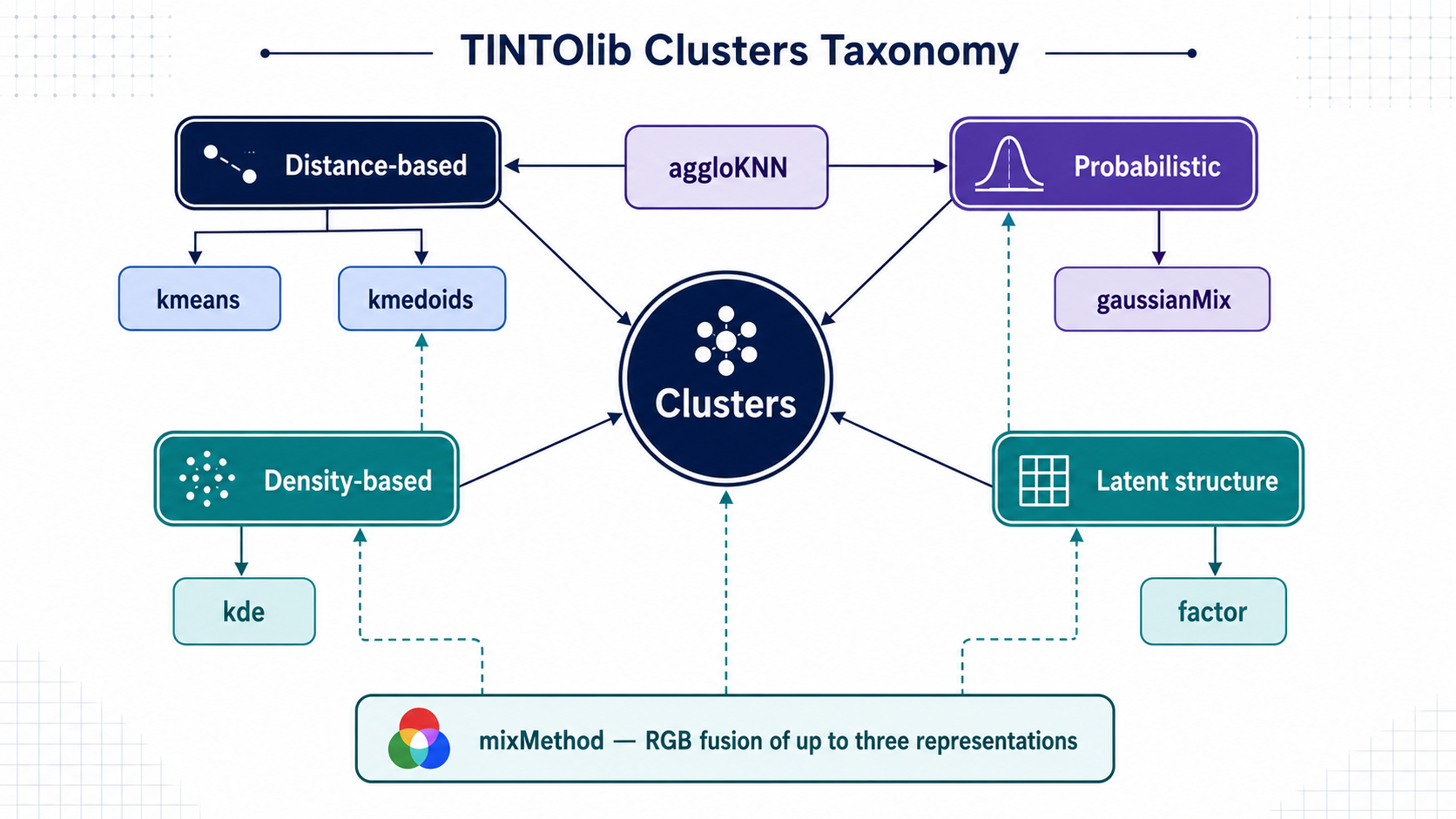
Available in mixMethod | Yes | No | Yes |
| Key interpretability caution | Component indices are arbitrary | Densities are feature-wise, not a joint sample probability | Pixel intensities hide the original score sign |
This table describes representational differences, not a performance ranking.
Practical implementation with a leakage-free split
The following example generates the three representations from the same Wine dataset split.
from pathlib import Path

import pandas as pd
from sklearn.datasets import load_wine
from sklearn.model_selection import train_test_split

from TINTOlib.clusters import Clusters

# ---------------------------------------------------------
# 1. Load a reproducible tabular dataset
# ---------------------------------------------------------
raw_data = load_wine()

df = pd.DataFrame(
    raw_data.data,
    columns=raw_data.feature_names
)

# The target column must be the final column.
df["target"] = raw_data.target

# ---------------------------------------------------------
# 2. Split before fitting any unsupervised transformation
# ---------------------------------------------------------
train_df, test_df = train_test_split(
    df,
    test_size=0.20,
    random_state=42,
    stratify=df["target"]
)

# ---------------------------------------------------------
# 3. Configure the three representations
# ---------------------------------------------------------
models = {
    "gaussianMix_full": Clusters(
        problem="classification",
        algorithm="gaussianMix",
        n_clusters=9,
        random_seed=1,
        n_init=5,
        max_iter=300,
        covariance_type="full"
    ),

    "kde_gaussian": Clusters(
        problem="classification",
        algorithm="kde",
        kernel="gaussian",
        bandwidth=0.5,
        metric="euclidean"
    ),

    "factor_9": Clusters(
        problem="classification",
        algorithm="factor",
        n_clusters=9,
        random_seed=1
    )
}

# ---------------------------------------------------------
# 4. Fit only on training data and reuse each fitted model
# ---------------------------------------------------------
for name, model in models.items():
    print(f"Generating images with {name}...")

    model.fit(train_df)

    train_folder = Path("synthetic_images") / name / "train"
    test_folder = Path("synthetic_images") / name / "test"

    model.transform(train_df, str(train_folder))
    model.transform(test_df, str(test_folder))

print("Probabilistic, density and latent images generated successfully.")
With these configurations:
gaussianMixgenerates nine responsibilities and therefore a $3\times3$ image;factorgenerates nine latent scores and therefore a $3\times3$ image;kdegenerates 13 density values for Wine and therefore a padded $4\times4$ image.
The image sizes are not automatically equivalent. A visual or predictive comparison must acknowledge this difference rather than resize or crop the representations without documenting the operation.
Exploring Gaussian covariance structures
Use the same split, sample and number of components when comparing covariance assumptions:
covariance_models = {
    covariance_type: Clusters(
        problem="classification",
        algorithm="gaussianMix",
        n_clusters=9,
        random_seed=1,
        n_init=5,
        max_iter=300,
        covariance_type=covariance_type
    )
    for covariance_type in [
        "full",
        "tied",
        "diag",
        "spherical"
    ]
}

for covariance_type, model in covariance_models.items():
    model.fit(train_df)

    model.transform(
        test_df,
        f"synthetic_images/gaussianMix_{covariance_type}/test"
    )
Do not compare images generated from independently changed splits or sample indices. Otherwise, visual differences cannot be attributed specifically to covariance_type.
Exploring KDE kernels and bandwidth
A controlled KDE experiment should vary one parameter at a time:
bandwidth_models = {
    f"gaussian_bw_{bandwidth}": Clusters(
        problem="classification",
        algorithm="kde",
        kernel="gaussian",
        bandwidth=bandwidth,
        metric="euclidean"
    )
    for bandwidth in [0.2, 0.5, 1.0, 2.0]
}

for name, model in bandwidth_models.items():
    model.fit(train_df)
    model.transform(
        test_df,
        f"synthetic_images/{name}/test"
    )
A separate kernel comparison can keep bandwidth=0.5 fixed and vary:
kernels = [
    "gaussian",
    "tophat",
    "epanechnikov",
    "exponential",
    "linear",
    "cosine"
]
Because KDE is applied separately to standardized one-dimensional features, bandwidth effects should be examined alongside the feature distributions rather than inferred only from the final image.
Exploring the number of latent factors
The factor count controls compression and image size:
factor_models = {
    f"factor_{n_factors}": Clusters(
        problem="classification",
        algorithm="factor",
        n_clusters=n_factors,
        random_seed=1
    )
    for n_factors in [4, 9, 12]
}

for name, model in factor_models.items():
    model.fit(train_df)
    model.transform(
        test_df,
        f"synthetic_images/{name}/test"
    )
For Wine, 12 is the maximum allowed value in the current implementation because the dataset contains 13 input features.
Same sample, different pixel semantics
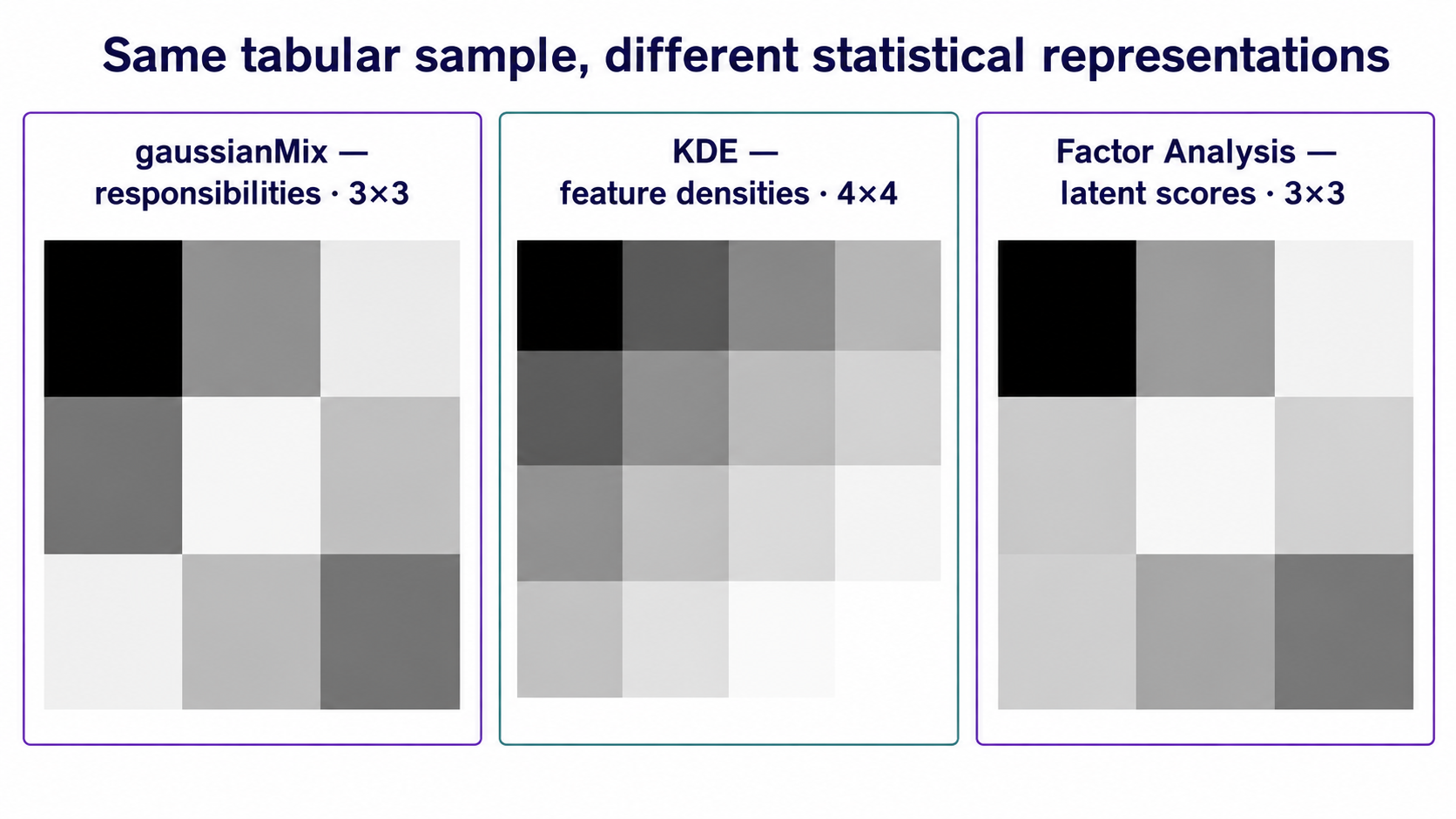 (Figure 5. Actual TINTOlib outputs generated from the same tabular sample using
 gaussianMix, kde and factor. The panels must preserve their native image dimensions and pixel values. Their visual patterns are not directly equivalent because they encode component responsibilities, feature-wise density estimates and latent-factor scores, respectively.)
A bright pixel has a method-dependent meaning:
| Method | Meaning before MinMax scaling | Meaning after image scaling |
|---|---|---|
gaussianMix | Large posterior responsibility for one component | High responsibility relative to the training range for that component |
kde | High estimated density for one feature value | High feature-wise density relative to the training scaling range |
factor | High signed score on one latent factor | High factor score relative to the training range, without retaining an explicit zero reference |
The same grayscale value therefore cannot be interpreted identically across methods.
Sparse, discrete and low-contrast images
Synthetic images generated by these methods can appear visually unusual.
gaussianMix
A nearly one-hot responsibility vector produces a highly discrete image. This may be a faithful representation of confident component assignment rather than a defective image.
kde
If several values lie in similarly dense regions, the image may have low contrast. Conversely, rare feature values can create sharp dark or bright differences after scaling, depending on the training density range.
factor
A small number of factors produces very compact images and potentially substantial padding. Increasing the number of factors changes both representational capacity and spatial dimensions.
Visual texture alone is not a sufficient quality criterion. Evaluation should include the intermediate numerical representation, image stability, predictive performance and computational cost.
Methodological checklist
Before comparing the three methods, verify that:
- the train/test split is created before fitting
Clusters; StandardScaler, Gaussian components, KDE estimators, factor projections and MinMax scalers are learned only from training data;- validation and test data are transformed without refitting;
- the same split and test sample are used in all visual comparisons;
- native image dimensions are reported;
- GMM covariance type, KDE kernel/bandwidth and factor count are documented;
- results are repeated across seeds when the method is stochastic;
- classical tabular baselines and an MLP remain part of the evaluation;
- CNN, ViT and hybrid models are compared under controlled settings;
- conclusions are conditional on the dataset and downstream architecture.
How should these representations be evaluated?
The experimental study that motivated these additions used regression, binary-classification and multiclass-classification datasets together with a particular Vision Transformer evaluation pipeline. Those results provide evidence for that experimental setting, but they do not establish a universal ordering among gaussianMix, kde, factor or the other transformations.
A representation may behave differently with:
- a convolutional neural network;
- a hybrid tabular–image architecture;
- another Vision Transformer configuration;
- a different image-resolution policy;
- another optimizer or regularization strategy;
- or a dataset with different dimensionality and distributional structure.
A rigorous comparison should therefore report:
- predictive metrics under identical data partitions;
- repeated runs and uncertainty estimates;
- transformation fit and generation time;
- memory and storage requirements;
- sensitivity to the main parameters;
- strong classical tabular and MLP baselines;
- results from more than one downstream visual architecture.
The objective of this tutorial is to explain what each method encodes, not to declare a universally superior transformation.
When should each representation be considered?
These are practical starting points rather than performance guarantees:
gaussianMixwhen soft membership, overlapping regions and component uncertainty are central to the analysis;kdewhen feature-wise commonness, rarity or local distributional structure is relevant;factorwhen a compact representation of shared covariance and latent structure is desired.
The choice should be validated empirically under the intended model and dataset.
Conclusion
gaussianMix, kde and factor transform the same tabular sample into three fundamentally different descriptions.
gaussianMixproduces posterior responsibilities over probabilistic components.kdeevaluates every feature value under its training distribution.factorprojects the sample onto latent dimensions that summarize shared variation.
TINTOlib converts all three representations into a common visual interface through training-based scaling, padding and square reshaping. That common output format should not obscure the fact that their pixels have different statistical meanings.
The final article in this series will examine RGB fusion through mixMethod, channel composition, interpretability and automatic structural-stability analysis using SSIM.
References and resources
Salvador Martínez Moreno. Generación de imágenes sintéticas mediante métodos no supervisados para la librería TINTOlib. Master’s Thesis, Universidad Nacional de Educación a Distancia (UNED), 2026.
TINTOlib documentation. Clusters. Read the current parameter and API documentation.
Research articles
Jiayun Liu, Manuel Castillo-Cara, Raúl García-Castro, Luis Orozco-Barbosa. Interpretable Hybrid Vision Transformer Architectures for MIMO-Based Indoor Localization using Synthetic Spatial Representations. IEEE Internet of Things. DOI: 10.1109/JIOT.2026.3696106
Jiayun Liu, Manuel Castillo-Cara, Raúl García-Castro. A Comprehensive Benchmark of Spatial Encoding Methods for Tabular Data with Deep Neural Networks. Information Fusion. DOI: 10.1016/j.inffus.2025.104088
Giovanny Mondragon-Ruiz, Jiayun Liu, Manuel Castillo-Cara, Raúl García-Castro. Interpretable CNN–KAN hybrid architectures for tabular data with synthetic image encoding. Information Processing and Management. DOI: 10.1016/j.ipm.2026.104954
Felipe Escalera-González, Manuel Castillo-Cara, Mariano Rincón-Zamorano, Luis Orozco-Barbosa. PermGrad: Interpretable Hybrid Neural Networks with synthetic images for tabular data. Knowledge-Based Systems. DOI: 10.1016/j.knosys.2026.116507
Manuel Castillo-Cara, Jesus Martínez-Gómez, Javier Ballesteros-Jerez, Ismael García-Varea, Raúl García-Castro, Luis Orozco-Barbosa. MIMO-Based Indoor Localisation with Hybrid Neural Networks. IEEE Journal of Selected Topics in Signal Processing. DOI: 10.1109/JSTSP.2025.3555067
Reewos Talla-Chumpitaz, Manuel Castillo-Cara, Luis Orozco-Barbosa, Raúl García-Castro. Blurring Image Techniques for Bluetooth-based Indoor Localisation. Information Fusion. DOI: 10.1016/j.inffus.2022.10.011
Software articles
Jiayun Liu, David González-Fernández, Manuel Castillo-Cara, Raúl García-Castro. TINTOlib: A Python library for transforming tabular data into synthetic images for deep neural networks. SoftwareX. DOI: 10.1016/j.softx.2025.102444
Manuel Castillo-Cara, Reewos Talla-Chumpitaz, Raúl García-Castro, Luis Orozco-Barbosa. TINTO: Converting Tidy Data into Image for Classification with 2-Dimensional Convolutional Neural Networks. SoftwareX. DOI: 10.1016/j.softx.2023.101391
Continue learning Artificial Intelligence
Explore practical courses on AI, Machine Learning, Deep Learning, Python, R and applied data science.

© Manuel Castillo-Cara, PhD. Content licensed under CC BY-NC 4.0 unless otherwise stated.