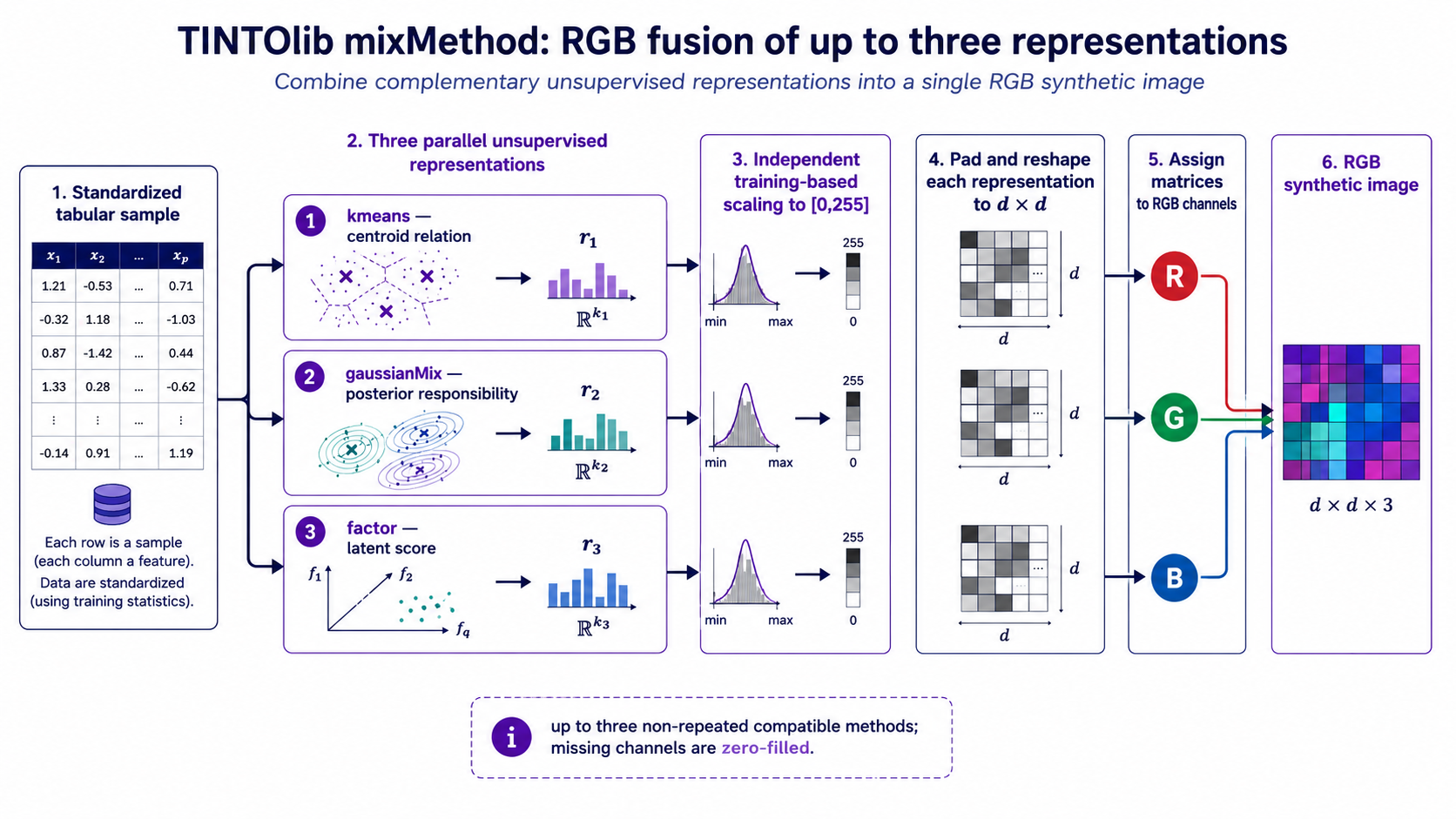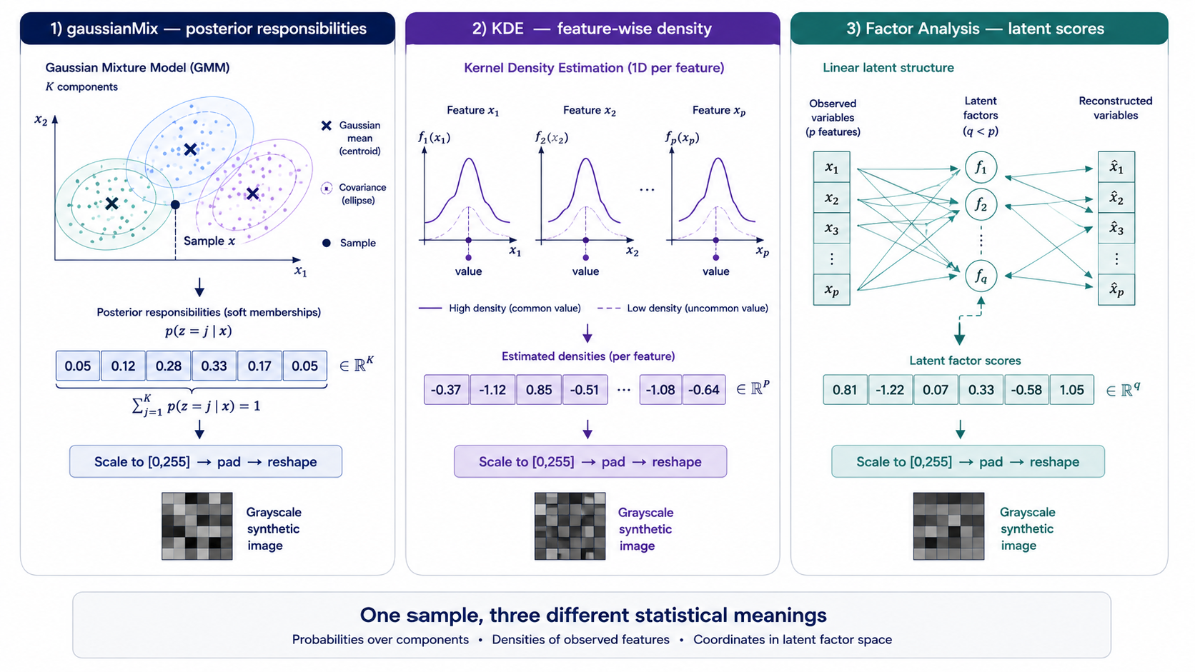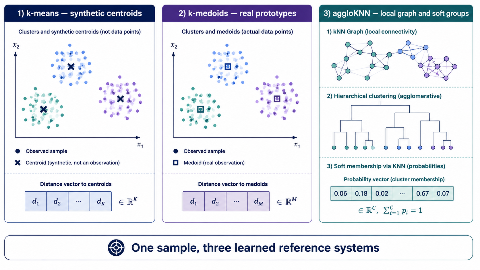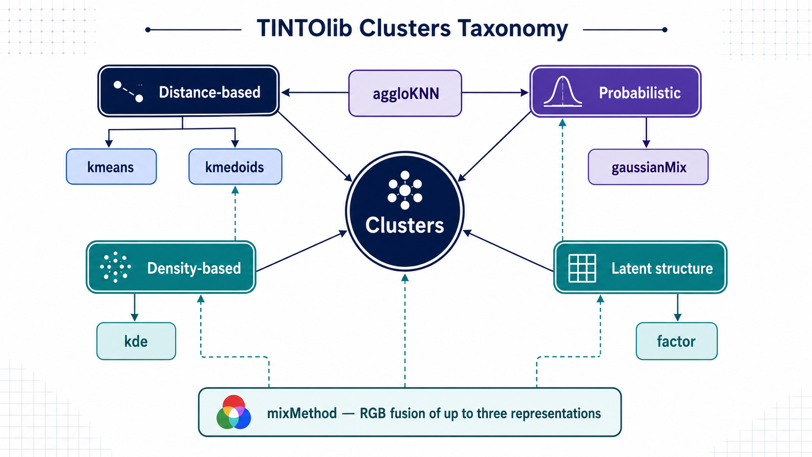
TINTOlib · Synthetic Images · Tabular-to-Image
What is TINTOlib?
Why does tabular data need spatial encoding? How are synthetic images generated — and what does blurring do? A complete introduction with a first end-to-end CNN pipeline in PyTorch.
- Author: Manuel Castillo-Cara, PhD
- Affiliation: Dpt. of Artificial Intelligence, Universidad Nacional de Educación a Distancia (UNED), Spain
- Role: Researcher, Professor, and TINTOlib Python Library Developer
- License: CC BY-NC 4.0 unless otherwise stated.
TINTOlib overview videos
The following short videos provide a bilingual introduction to TINTOlib, explaining how tabular data can be transformed into synthetic images and processed with computer vision architectures such as CNNs, Vision Transformers and hybrid neural networks.
In many applied machine learning problems, there is a recurrent practical distinction: for images, text, or audio, we often use Deep Learning; for tabular data, tree-based models and ensembles such as Random Forest, XGBoost, LightGBM, or CatBoost remain extremely competitive.
This distinction is not accidental. Convolutional neural networks were designed to exploit spatial structure: local neighborhoods, edges, textures, shapes, and patterns that repeat across an image. A tabular dataset, however, does not naturally have this type of geometry. The fact that one variable appears in column 2 and another in column 3 does not imply that both variables are semantically or statistically close.
This leads to a relevant research question:
Can we transform each tabular instance into a synthetic image so that computer vision architectures can exploit relationships between variables?
This question motivates the field of tabular-to-image transformation, also referred to as tabular2image, spatial encoding for tabular data, or synthetic image generation from tabular data. In this post, we introduce the main idea, explain where TINTOlib fits, and build a simple convolutional neural network in PyTorch to classify synthetic images generated from tabular data.
The problem: tabular data has no natural spatial locality
A digital image can be represented as a matrix of pixels. In a natural image, nearby pixels usually belong to the same visual region: an edge, a texture, a shadow, or an object. This property allows CNNs to apply local filters and learn reusable spatial patterns.
A tabular instance is different. It is usually represented as a vector:
x = [age, blood_pressure, cholesterol, glucose, ...]
The order of the columns is often arbitrary. If two variables are swapped, the semantic meaning of the sample does not necessarily change. For a CNN, however, that change would modify the input geometry. This is one of the reasons why applying convolutions directly to tabular vectors is usually problematic: the model would assume a local neighborhood structure that is not explicitly present.
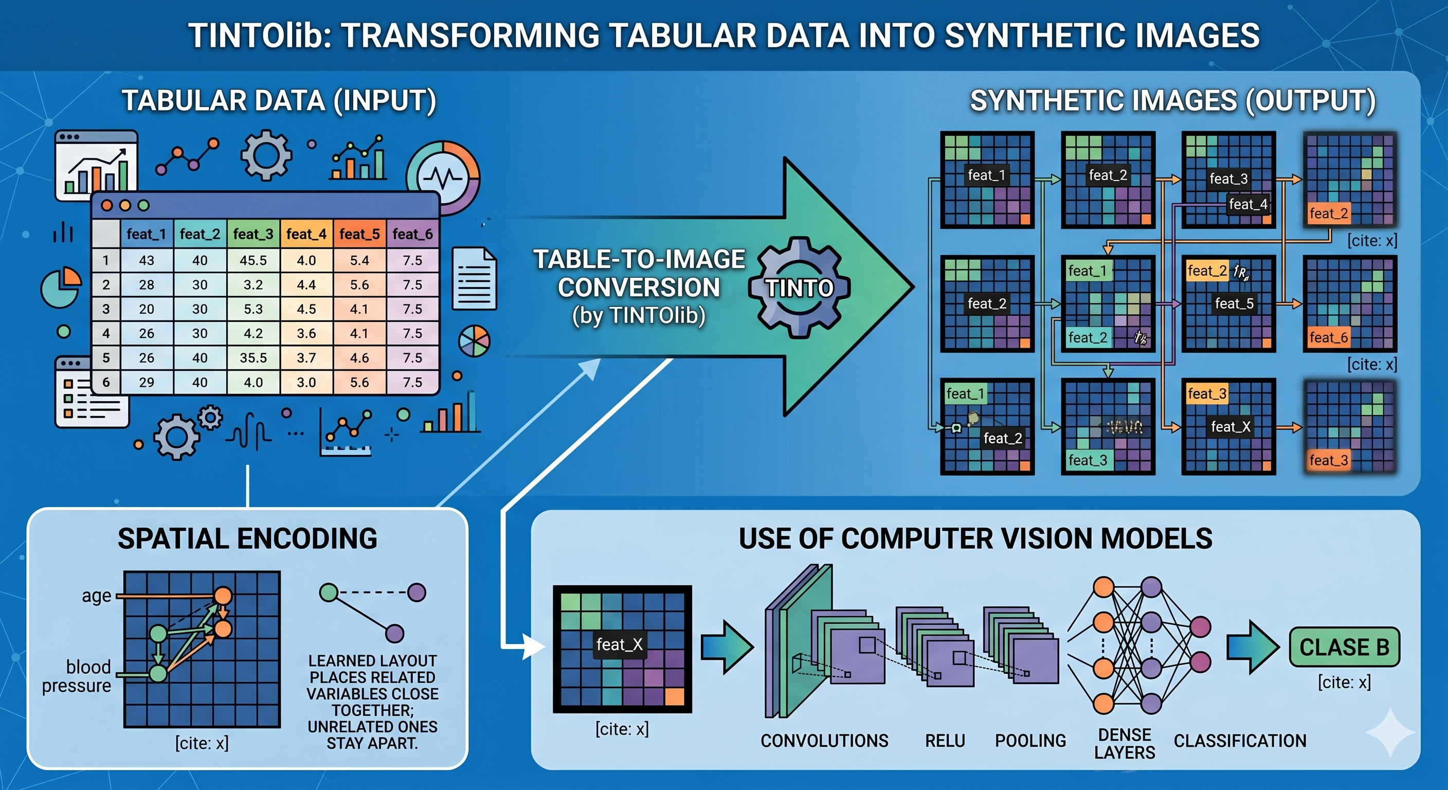
Tabular-to-image transformation addresses this limitation by constructing an artificial spatial layout. The idea is to place the original variables on a 2D grid so that related variables are positioned close to each other. Then, for each row in the dataset, the values of those variables are projected onto the grid, producing a synthetic image.
Tabular data                    Synthetic image

+--------+--------+--------+       +----+----+----+----+
| feat_1 | feat_2 | feat_3 |  -->  |    | f2 |    | f8 |
| feat_4 | feat_5 | feat_6 |       +----+----+----+----+
|  ...   |  ...   |  ...   |       | f1 |    | f5 |    |
+--------+--------+--------+       +----+----+----+----+
                                   |    | f3 | f4 |    |
                                   +----+----+----+----+
(Conceptual schematic of the transformation from tabular data to a synthetic 2D image. Each feature is mapped to a grid position such that related variables are placed close to each other.)
This image is not a natural image. It does not represent a real-world scene. It is a spatial representation of a tabular vector. The important point is not whether the image is visually meaningful to a human observer, but whether the representation encodes useful relationships for a vision-based model.
(Figure 1. Conceptual workflow of TINTOlib for transforming tabular data into synthetic images. The original tabular features are spatially encoded into a two-dimensional grid, producing image-like representations that preserve feature relationships and can be processed by computer vision models such as convolutional neural networks.)
Why transform tabular data into images?
The transformation of tabular data into synthetic images opens at least three relevant possibilities.
First, it allows us to use computer vision architectures on structured data. Once each tabular instance has been transformed into an image, we can use CNNs, Vision Transformers, pretrained backbones, or hybrid neural architectures.
Second, it introduces a spatial inductive bias. If the transformation method places related variables close to each other, convolutional filters can learn local interactions between features.
Third, it enables visual explainability techniques. Methods such as saliency maps, activation maps, or Grad-CAM can be adapted to study which regions of the synthetic image — and therefore which original variables — contributed most to the prediction.
This does not mean that tabular-to-image transformation will always outperform classical machine learning models. Tree-based models remain strong baselines for tabular data. The value of this approach depends on the dataset, the number of samples, the number of features, the transformation method, the neural architecture, and the evaluation protocol. Its main interest is that it provides an alternative representation that can be combined with modern vision-based deep learning methods.
What is TINTOlib?
TINTOlib is a Python library for transforming tabular data into synthetic images in a systematic, modular, and reproducible way. Its main goal is to provide a unified interface for different state-of-the-art tabular-to-image transformation methods that were previously scattered across independent implementations, often with heterogeneous APIs.
The library follows a Scikit-Learn-like design, including methods such as fit, transform, and fit_transform. This is particularly useful when designing machine learning pipelines, because it allows us to separate the learning of the spatial representation from the transformation of new data.
TINTOlib includes both parametric and non-parametric methods. Some examples are:
- TINTO, based on dimensionality reduction techniques such as PCA or t-SNE, with optional image blurring.
- IGTD, which optimizes the feature arrangement to preserve similarity relationships.
- REFINED, which relies on multidimensional scaling and optimization to preserve feature-neighborhood information.
- DeepInsight, another projection-based method that arranges features in a 2D space.
- BarGraph, DistanceMatrix, Combination, FeatureWrap, SuperTML, and BIE, among others.
The documentation is available at tintolib.readthedocs.io.
The source code and examples are available at github.com/oeg-upm/TINTOlib.
In practice, TINTOlib allows us to move from this representation:
samples x features
to this one:
samples x channels x height x width
which is the natural input format for computer vision models in PyTorch.
Avoiding data leakage: fit only on the training data
A critical point when using tabular-to-image methods is data leakage.
The spatial arrangement of the variables must be learned only from the training data. If we use the full dataset to learn the transformation — including validation or test samples — information from the evaluation split can indirectly influence the representation. This would lead to an optimistic and methodologically incorrect estimate of model performance.
Therefore, even though TINTOlib provides fit_transform for convenience, in a proper experimental pipeline we should use:
fiton the training set only;transformon the training set;transformon the validation and test sets using the already-fitted transformation.
Conceptually, the workflow should be:
Train tabular data  ---- fit ----> learned spatial layout
Train tabular data  -- transform -> train images
Validation data     -- transform -> validation images
Test data           -- transform -> test images
This is the same principle used with scalers, imputers, PCA, feature selectors, and other preprocessing methods in standard machine learning pipelines.
First practical example: generating synthetic images with TINTOlib
For this example, we consider a multiclass classification problem using the Wine dataset from Scikit-Learn. Each row represents a sample, the input columns are numerical features, and the target column identifies the class label.
Install TINTOlib with:
pip install TINTOlib
Then, we prepare the train, validation, and test splits before fitting the tabular-to-image transformation.
from pathlib import Path

import pandas as pd
from sklearn.datasets import load_wine
from sklearn.model_selection import train_test_split
from sklearn.preprocessing import LabelEncoder

from TINTOlib.tinto import TINTO

# Reproducibility
seed = 42

# Load multiclass tabular dataset
raw_data = load_wine()

# Build dataframe
df = pd.DataFrame(raw_data.data, columns=raw_data.feature_names)
df["target"] = raw_data.target

# Separate features and target
target_col = "target"
X = df.drop(columns=[target_col])
y = df[target_col]

# Encode labels if needed
label_encoder = LabelEncoder()
y_encoded = label_encoder.fit_transform(y)

# First split: train + temporary set
X_train, X_tmp, y_train, y_tmp = train_test_split(
    X,
    y_encoded,
    test_size=0.30,
    random_state=seed,
    stratify=y_encoded
)

# Second split: validation + test
X_val, X_test, y_val, y_test = train_test_split(
    X_tmp,
    y_tmp,
    test_size=0.50,
    random_state=seed,
    stratify=y_tmp
)

# Rebuild dataframes because TINTOlib expects the target column together with the features
train_df = X_train.copy()
train_df[target_col] = y_train

val_df = X_val.copy()
val_df[target_col] = y_val

test_df = X_test.copy()
test_df[target_col] = y_test
Now we instantiate the TINTO transformation. In this example we use the TINTO method, but the same structure can be used with other TINTOlib methods such as IGTD, REFINED, DeepInsight, BarGraph, DistanceMatrix, SuperTML, or BIE.
# Output folders
output_root = Path("tinto_images")
train_folder = output_root / "train"
val_folder = output_root / "val"
test_folder = output_root / "test"

# TINTO model
# pixels defines the image size: pixels x pixels
image_model = TINTO(
    problem="supervised",
    algorithm="PCA",
    pixels=20,
    blur=True,
    random_seed=seed
)

# Learn the spatial layout ONLY from the training data
image_model.fit(train_df)

# Transform each split using the same fitted representation
image_model.transform(train_df, folder=str(train_folder))
image_model.transform(val_df, folder=str(val_folder))
image_model.transform(test_df, folder=str(test_folder))

print("Synthetic images generated successfully.")
This separation is essential. The validation and test sets are transformed using the spatial layout learned from the training data, but they do not participate in learning that layout.


(Figure 2. Synthetic image samples generated with TINTOlib using the TINTO method with blurring, showing one representative instance from each class of the Wine multiclass dataset. Each image corresponds to a different class and encodes the original tabular feature values into a two-dimensional spatial representation, where local smoothing enhances spatial continuity while preserving class-dependent patterns that can be exploited by CNN-based and hybrid deep learning models.)
Can we use another method instead of TINTO?
Yes. One of the main advantages of TINTOlib is that the same general workflow can be reused with different transformation methods. For example, depending on the method available in your installation, you could replace the import and model definition with another transformer:
# Example: using another TINTOlib method instead of TINTO
# from TINTOlib.igtd import IGTD
# image_model = IGTD(problem="supervised", pixels=20)

# from TINTOlib.refined import REFINED
# image_model = REFINED(problem="supervised", pixels=20)
The high-level logic remains the same:
image_model.fit(train_df)
image_model.transform(train_df, folder="...")
image_model.transform(val_df, folder="...")
image_model.transform(test_df, folder="...")
For an experimental paper or benchmark, this is particularly useful because it allows us to compare different spatial encodings while keeping the same downstream neural architecture.
Loading the generated images in PyTorch
Once the images have been generated, we can load them in PyTorch. The exact folder structure may depend on the selected TINTOlib method and configuration. For a simple classification pipeline, it is convenient to organize the images using the structure expected by torchvision.datasets.ImageFolder:
tinto_images/
├── train/
│   ├── class_0/
│   ├── class_1/
│   └── class_2/
├── val/
│   ├── class_0/
│   ├── class_1/
│   └── class_2/
└── test/
    ├── class_0/
    ├── class_1/
    └── class_2/
If your generated files are stored differently, you can either reorganize them into this structure or implement a custom PyTorch Dataset.
import torch
from torch.utils.data import DataLoader
from torchvision import datasets, transforms

batch_size = 32
img_size = 20

transform = transforms.Compose([
    transforms.Grayscale(num_output_channels=1),
    transforms.Resize((img_size, img_size)),
    transforms.ToTensor(),
])

train_dataset = datasets.ImageFolder(root=train_folder, transform=transform)
val_dataset = datasets.ImageFolder(root=val_folder, transform=transform)
test_dataset = datasets.ImageFolder(root=test_folder, transform=transform)

num_classes = len(train_dataset.classes)

train_loader = DataLoader(
    train_dataset,
    batch_size=batch_size,
    shuffle=True,
    num_workers=2
)

val_loader = DataLoader(
    val_dataset,
    batch_size=batch_size,
    shuffle=False,
    num_workers=2
)

test_loader = DataLoader(
    test_dataset,
    batch_size=batch_size,
    shuffle=False,
    num_workers=2
)

print("Classes:", train_dataset.classes)
print("Number of classes:", num_classes)
print("Training images:", len(train_dataset))
print("Validation images:", len(val_dataset))
print("Test images:", len(test_dataset))
A simple CNN in PyTorch
The following network defines a compact CNN baseline for verifying that the synthetic images generated by TINTOlib can be loaded, processed, and classified within a standard PyTorch workflow.
We assume grayscale images of size 20 x 20 pixels.
import torch
import torch.nn as nn


class SimpleTINTOCNN(nn.Module):
    def __init__(self, num_classes: int, img_size: int = 20):
        super().__init__()

        self.features = nn.Sequential(
            nn.Conv2d(in_channels=1, out_channels=32, kernel_size=3, padding=1),
            nn.ReLU(),
            nn.MaxPool2d(kernel_size=2),

            nn.Conv2d(in_channels=32, out_channels=64, kernel_size=3, padding=1),
            nn.ReLU(),
            nn.MaxPool2d(kernel_size=2),
        )

        # For img_size=20: 20 -> 10 -> 5 after two MaxPool2d layers
        reduced_size = img_size // 4

        self.classifier = nn.Sequential(
            nn.Flatten(),
            nn.Linear(64 * reduced_size * reduced_size, 128),
            nn.ReLU(),
            nn.Dropout(p=0.3),
            nn.Linear(128, num_classes)
        )

    def forward(self, x):
        x = self.features(x)
        x = self.classifier(x)
        return x


device = torch.device("cuda" if torch.cuda.is_available() else "cpu")

model = SimpleTINTOCNN(num_classes=num_classes, img_size=img_size).to(device)
print(model)
Training the model
For multiclass classification, we use CrossEntropyLoss. In PyTorch, this loss expects raw logits, so the final layer should not include a softmax activation.
import torch.optim as optim

criterion = nn.CrossEntropyLoss()
optimizer = optim.Adam(model.parameters(), lr=1e-3)


def train_one_epoch(model, dataloader, criterion, optimizer, device):
    model.train()
    running_loss = 0.0
    correct = 0
    total = 0

    for images, labels in dataloader:
        images = images.to(device)
        labels = labels.to(device)

        optimizer.zero_grad()
        outputs = model(images)
        loss = criterion(outputs, labels)
        loss.backward()
        optimizer.step()

        running_loss += loss.item() * images.size(0)
        predictions = outputs.argmax(dim=1)
        correct += (predictions == labels).sum().item()
        total += labels.size(0)

    epoch_loss = running_loss / total
    epoch_acc = correct / total

    return epoch_loss, epoch_acc


@torch.no_grad()
def evaluate(model, dataloader, criterion, device):
    model.eval()
    running_loss = 0.0
    correct = 0
    total = 0

    for images, labels in dataloader:
        images = images.to(device)
        labels = labels.to(device)

        outputs = model(images)
        loss = criterion(outputs, labels)

        running_loss += loss.item() * images.size(0)
        predictions = outputs.argmax(dim=1)
        correct += (predictions == labels).sum().item()
        total += labels.size(0)

    epoch_loss = running_loss / total
    epoch_acc = correct / total

    return epoch_loss, epoch_acc
Now we train the network.
num_epochs = 20

history = {
    "train_loss": [],
    "train_acc": [],
    "val_loss": [],
    "val_acc": [],
}

for epoch in range(num_epochs):
    train_loss, train_acc = train_one_epoch(
        model,
        train_loader,
        criterion,
        optimizer,
        device
    )

    val_loss, val_acc = evaluate(
        model,
        val_loader,
        criterion,
        device
    )

    history["train_loss"].append(train_loss)
    history["train_acc"].append(train_acc)
    history["val_loss"].append(val_loss)
    history["val_acc"].append(val_acc)

    print(
        f"Epoch [{epoch + 1:02d}/{num_epochs}] "
        f"Train Loss: {train_loss:.4f} | Train Acc: {train_acc:.4f} | "
        f"Val Loss: {val_loss:.4f} | Val Acc: {val_acc:.4f}"
    )
Evaluating on the test set
The test set should only be used once the model selection process has finished. Here we report the final test performance using the model selected during validation.
test_loss, test_acc = evaluate(model, test_loader, criterion, device)

print(f"Test Loss: {test_loss:.4f}")
print(f"Test Accuracy: {test_acc:.4f}")
Visualizing the training curves
In a Jupyter notebook, it is useful to visualize the learning curves to check whether the model is learning and whether overfitting appears.
import matplotlib.pyplot as plt

plt.figure(figsize=(7, 4))
plt.plot(history["train_loss"], label="Train loss")
plt.plot(history["val_loss"], label="Validation loss")
plt.xlabel("Epoch")
plt.ylabel("Loss")
plt.title("Training and validation loss")
plt.legend()
plt.grid(True)
plt.show()

plt.figure(figsize=(7, 4))
plt.plot(history["train_acc"], label="Train accuracy")
plt.plot(history["val_acc"], label="Validation accuracy")
plt.xlabel("Epoch")
plt.ylabel("Accuracy")
plt.title("Training and validation accuracy")
plt.legend()
plt.grid(True)
plt.show()
Visualizing synthetic images
It is also useful to inspect some generated images. This helps to emphasize that these are not natural images, but artificial spatial encodings of tabular samples.
images, labels = next(iter(train_loader))

plt.figure(figsize=(10, 4))
for i in range(min(8, images.size(0))):
    plt.subplot(2, 4, i + 1)
    plt.imshow(images[i].squeeze(0), cmap="gray")
    plt.title(f"Class: {labels[i].item()}")
    plt.axis("off")

plt.tight_layout()
plt.show()
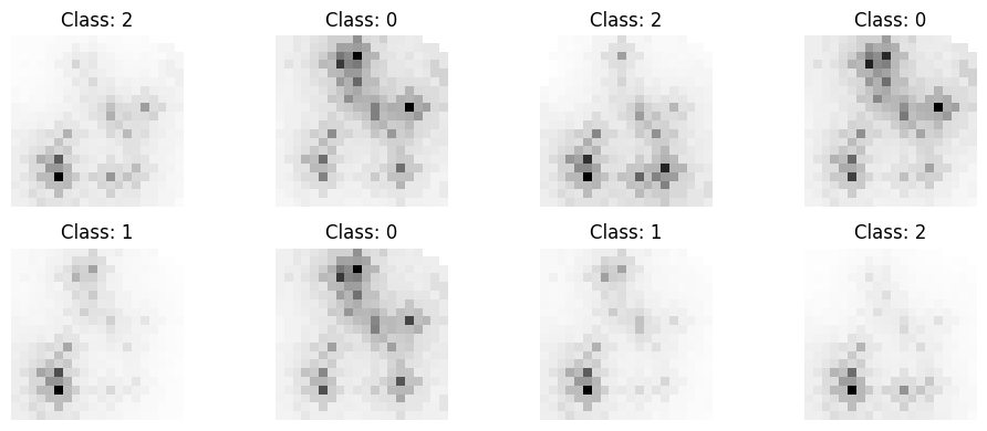 (Figure 3. Visualization of a batch of synthetic images generated with TINTOlib using the TINTO method with blurring. Each panel represents an individual tabular sample from the Wine dataset, encoded as a grayscale two-dimensional image and labeled according to its class. The observed spatial intensity patterns illustrate how different classes may produce distinguishable synthetic representations that can be processed by CNN-based models.)
What should we compare next?
This first experiment trains a simple CNN, but a rigorous evaluation should include additional baselines and ablations:
- a classical machine learning baseline, such as Random Forest, XGBoost, LightGBM, or CatBoost;
- a multilayer perceptron trained on the original tabular data;
- different tabular-to-image transformations, such as TINTO, IGTD, REFINED, DeepInsight, and SuperTML;
- different image sizes;
- deeper CNNs or Vision Transformers;
- hybrid architectures combining a tabular branch and an image branch.
The main question is not only whether a CNN can outperform a tree-based model. The scientifically relevant question is when, why, and under which conditions a spatial representation of tabular data is beneficial.
Conclusion
TINTOlib makes it easier to experiment with a powerful idea: transforming tabular data into visual representations that can be processed by computer vision architectures. This transformation does not automatically make a tabular problem easier, but it provides a different representation where spatial inductive biases can be exploited.
The key element is the spatial arrangement of the features. If related variables are placed close to each other, CNN filters can learn local interactions that are not directly available in the original table. In addition, this representation enables hybrid architectures, Vision Transformers, and visual explainability methods for structured data.
In this post, we introduced the motivation behind tabular-to-image transformation, the role of TINTOlib, the importance of avoiding data leakage, and a first CNN implementation in PyTorch. In future posts, we will compare different TINTOlib methods, build hybrid tabular-image neural networks, and apply explainability techniques to recover the relevance of the original variables.
References and related publications
The concepts presented in this tutorial are connected to the following research and software publications on TINTO, TINTOlib, tabular-to-image transformation, synthetic spatial representations, hybrid neural networks, and indoor localisation.
Research articles
Jiayun Liu, Manuel Castillo-Cara, Raúl García-Castro, Luis Orozco-Barbosa. Interpretable Hybrid Vision Transformer Architectures for MIMO-Based Indoor Localization using Synthetic Spatial Representations. IEEE Internet of Things. DOI: 10.1109/JIOT.2026.3696106
Jiayun Liu, Manuel Castillo-Cara, Raúl García-Castro. A Comprehensive Benchmark of Spatial Encoding Methods for Tabular Data with Deep Neural Networks. Information Fusion. DOI: 10.1016/j.inffus.2025.104088
Giovanny Mondragon-Ruiz, Jiayun Liu, Manuel Castillo-Cara, Raúl García-Castro. Interpretable CNN–KAN hybrid architectures for tabular data with synthetic image encoding. Information Processing and Management. DOI: 10.1016/j.ipm.2026.104954
Felipe Escalera-González, Manuel Castillo-Cara, Mariano Rincón-Zamorano, Luis Orozco-Barbosa. PermGrad: Interpretable Hybrid Neural Networks with synthetic images for tabular data. Knowledge-Based Systems. DOI: 10.1016/j.knosys.2026.116507
Manuel Castillo-Cara, Jesus Martínez-Gómez, Javier Ballesteros-Jerez, Ismael García-Varea, Raúl García-Castro, Luis Orozco-Barbosa. MIMO-Based Indoor Localisation with Hybrid Neural Networks. IEEE Journal of Selected Topics in Signal Processing. DOI: 10.1109/JSTSP.2025.3555067
Reewos Talla-Chumpitaz, Manuel Castillo-Cara, Luis Orozco-Barbosa, Raúl García-Castro. Blurring Image Techniques for Bluetooth-based Indoor Localisation. Information Fusion. DOI: 10.1016/j.inffus.2022.10.011
Software articles
Jiayun Liu, David González-Fernández, Manuel Castillo-Cara, Raúl García-Castro. TINTOlib: A Python library for transforming tabular data into synthetic images for deep neural networks. SoftwareX. DOI: 10.1016/j.softx.2025.102444
Manuel Castillo-Cara, Reewos Talla-Chumpitaz, Raúl García-Castro, Luis Orozco-Barbosa. TINTO: Converting Tidy Data into Image for Classification with 2-Dimensional Convolutional Neural Networks. SoftwareX. DOI: 10.1016/j.softx.2023.101391
Continue learning Artificial Intelligence
Explore practical courses on AI, Machine Learning, Deep Learning, Python, R and applied data science.

© Manuel Castillo-Cara, PhD. Content licensed under CC BY-NC 4.0 unless otherwise stated.